Texas Instruments TI-36X Pro User Manual - Page 37
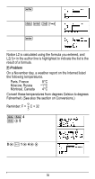
For four points, the equation - linear regression
 |
View all Texas Instruments TI-36X Pro manuals
Add to My Manuals
Save this manual to your list of manuals |
Page 37 highlights
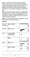
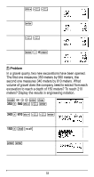
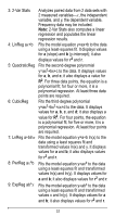
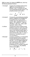
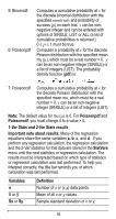
3: 2-Var Stats Analyzes paired data from 2 data sets with 2 measured variables-x, the independent variable, and y, the dependent variable. Frequency data may be included. Note: 2-Var Stats also computes a linear regression and populates the linear regression results. 4: LinReg ax+b Fits the model equation y=ax+b to the data using a least-squares fit. It displays values for a (slope) and b (y-intercept); it also displays values for r2 and r. 5: QuadraticReg Fits the second-degree polynomial y=ax2+bx+c to the data. It displays values for a, b, and c; it also displays a value for R2. For three data points, the equation is a polynomial fit; for four or more, it is a polynomial regression. At least three data points are required. 6: CubicReg Fits the third-degree polynomial y=ax3+bx2+cx+d to the data. It displays values for a, b, c, and d; it also displays a value for R2. For four points, the equation is a polynomial fit; for five or more, it is a polynomial regression. At least four points are required. 7: LnReg a+blnx Fits the model equation y=a+b ln(x) to the data using a least squares fit and transformed values ln(x) and y. It displays values for a and b; it also displays values for r2 and r. 8: PwrReg ax^b Fits the model equation y=axb to the data using a least-squares fit and transformed values ln(x) and ln(y). It displays values for a and b; it also displays values for r2 and r. 9: ExpReg ab^x Fits the model equation y=abx to the data using a least-squares fit and transformed values x and ln(y). It displays values for a and b; it also displays values for r2 and r. 37
-
 1
1 -
2
-
3
-
4
-
5
-
6
-
7
-
8
-
9
-
10
-
11
-
12
-
13
-
14
-
15
-
16
-
17
-
18
-
19
-
20
-
21
-
22
-
23
-
24
-
25
-
26
-
27
-
28
-
29
-
30
-
31
-
 32
32 -
 33
33 -
 34
34 -
 35
35 -
 36
36 -
 37
37 -
 38
38 -
 39
39 -
 40
40 -
 41
41 -
 42
42 -
43
-
44
-
45
-
46
-
47
-
48
-
49
-
50
-
51
-
52
-
53
-
54
-
55
-
56
-
57
-
58
-
59
-
60
-
61
-
62
-
63
-
64
-
65
-
66
-
67
-
68
-
69
-
70
-
71
-
72
-
73
-
74
-
75
-
76
-
77
-
78
 |
 |
