HP ProLiant 4000 Disk Subsystem Performance and Scalability - Page 8

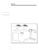
WHITE PAPER (cont.) Note: Remember that the disks used in Figure 2 are identical in size and RAID configuration. ECG025.0997 ... However, be aware that the average latency time might not always decrease when adding more drives to your system. For example, in Figure 2 - Example 2, the new configuration shows that the amount of time it takes to retrieve the data from sector B is actually longer than the initial configuration. The reason for this is that the disk has to spin half way around to read sector B. In the initial configuration the disk only had to spin one-eighth a revolution to read the identical data. But, keep in mind that the initial configuration for Example 2 required both seek time and latency time. Initial Configuration Example 1 4 D 3C 5 E F6 2B A 1 G7 H Example 2 8 New Configuration 7 5 A C 3 1 Example 1 E G Disk Head Example 2 8 6 4 2 B D F H Disk Head Disk Head Figure 2: Average Latency Overall, these examples show us that in some configurations, as shown in our first example, drive scaling would be a definite performance advantage. However, in other configurations it is not clear if you receive a performance gain because of the components involved, such as the combination of average seek time and average latency time used in Figure 2 - Example 2. When you combine these terms (average seek time and average latency time), you define another disk measurement called average access time, which is discussed in the upcoming section. From the information provided in this section, we know seek time plus latency (or average access time) is a key in determining if performance is truly enhanced in your system. 8