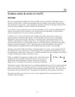
HP 39GS HP 39gs_40gs_Mastering The Graphing Calculator_English_E_F2224-90010.p - Page 235
matrices they should investigate.
 |
UPC - 808736931328
View all HP 39GS manuals
Add to My Manuals
Save this manual to your list of manuals |
Page 235 highlights
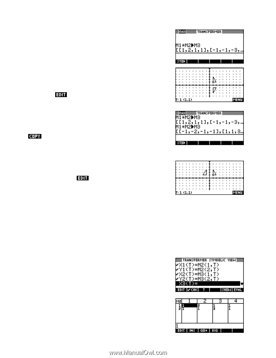
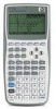
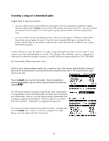
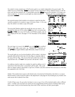
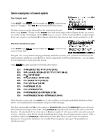
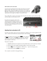
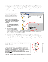
Change to the HOME view and perform the calculation shown right and finally press PLOT. The result is a triangle with corners at (1,1), (2,1) and (1,3), along with its image after reflection in the x axis. We can now matrix M1 so that it contains another matrix. ⎡−1 0⎤ For example: ⎢ ⎢ ⎣ 0 1⎥⎦⎥ To see the effect of this new matrix, simply return to the HOME view, the previous calculation and press ENTER. The new image will be stored into matrix M3. If you now return to the PLOT view the image will not appear to have changed as the aplet does not realize the matrix has changed but pressing PLOT again will force a re-draw of the new image. The great power of this aplet is its use as a teaching and investigative tool. Simply continue to matrix M1, repeating the HOME calculation, and re-PLOTing each time to see the change in the image. For teachers, the degree of guidance which should be given to a class will obviously depend on their level of ability. For an able class you might choose to give no more guidance than to suggest that they confine their investigations initially to placing numbers only on the diagonals. It may be a good idea to challenge them to record their matrices on the board as they discovered them. For a less able class you might hand out a list of matrices they should investigate. Perhaps in the form of a set of cards with matrices and geometric trans formations which must be matched up. A highly able class will find nearly all relevant matrices within 20 to 30 minutes. A less able class may need considerable guidance. So... how does this aplet work? The formulas in the SYMB view form the key to the process by allowing the calculator to fetch values from the matrices, with the values fetched being determined by the settings in the PLOT SETUP view. For example, as T runs from 1 to 4 in steps of 1 the (X1,Y1) values plotted become (M2(1,1),M2(2,1)), (M2(1,2),M2(2,2)), (M2(1,3),M2(2,3)) and (M2(1,4),M2(2,4)). If we now substitute the actual values from matrix M2 then these points become (1,1), (2,1), (3,1) and (1,1), which give the shape when plotted. 235
-
 1
1 -
2
-
3
-
4
-
5
-
6
-
7
-
8
-
9
-
10
-
11
-
12
-
13
-
14
-
15
-
16
-
17
-
18
-
19
-
20
-
21
-
22
-
23
-
24
-
25
-
26
-
27
-
28
-
29
-
30
-
31
-
32
-
33
-
34
-
35
-
36
-
37
-
38
-
39
-
40
-
41
-
42
-
43
-
44
-
45
-
46
-
47
-
48
-
49
-
50
-
51
-
52
-
53
-
54
-
55
-
56
-
57
-
58
-
59
-
60
-
61
-
62
-
63
-
64
-
65
-
66
-
67
-
68
-
69
-
70
-
71
-
72
-
73
-
74
-
75
-
76
-
77
-
78
-
79
-
80
-
81
-
82
-
83
-
84
-
85
-
86
-
87
-
88
-
89
-
90
-
91
-
92
-
93
-
94
-
95
-
96
-
97
-
98
-
99
-
100
-
101
-
102
-
103
-
104
-
105
-
106
-
107
-
108
-
109
-
110
-
111
-
112
-
113
-
114
-
115
-
116
-
117
-
118
-
119
-
120
-
121
-
122
-
123
-
124
-
125
-
126
-
127
-
128
-
129
-
130
-
131
-
132
-
133
-
134
-
135
-
136
-
137
-
138
-
139
-
140
-
141
-
142
-
143
-
144
-
145
-
146
-
147
-
148
-
149
-
150
-
151
-
152
-
153
-
154
-
155
-
156
-
157
-
158
-
159
-
160
-
161
-
162
-
163
-
164
-
165
-
166
-
167
-
168
-
169
-
170
-
171
-
172
-
173
-
174
-
175
-
176
-
177
-
178
-
179
-
180
-
181
-
182
-
183
-
184
-
185
-
186
-
187
-
188
-
189
-
190
-
191
-
192
-
193
-
194
-
195
-
196
-
197
-
198
-
199
-
200
-
201
-
202
-
203
-
204
-
205
-
206
-
207
-
208
-
209
-
210
-
211
-
212
-
213
-
214
-
215
-
216
-
217
-
218
-
219
-
220
-
221
-
222
-
223
-
224
-
225
-
226
-
227
-
228
-
229
-
 230
230 -
 231
231 -
 232
232 -
 233
233 -
 234
234 -
 235
235 -
 236
236 -
 237
237 -
 238
238 -
 239
239 -
 240
240 -
241
-
242
-
243
-
244
-
245
-
246
-
247
-
248
-
249
-
250
-
251
-
252
-
253
-
254
-
255
-
256
-
257
-
258
-
259
-
260
-
261
-
262
-
263
-
264
-
265
-
266
-
267
-
268
-
269
-
270
-
271
-
272
-
273
-
274
-
275
-
276
-
277
-
278
-
279
-
280
-
281
-
282
-
283
-
284
-
285
-
286
-
287
-
288
-
289
-
290
-
291
-
292
-
293
-
294
-
295
-
296
-
297
-
298
-
299
-
300
-
301
-
302
-
303
-
304
-
305
-
306
-
307
-
308
-
309
-
310
-
311
-
312
-
313
-
314
-
315
-
316
-
317
-
318
-
319
-
320
-
321
-
322
-
323
-
324
-
325
-
326
-
327
-
328
-
329
-
330
-
331
-
332
-
333
-
334
-
335
-
336
-
337
-
338
-
339
-
340
-
341
-
342
-
343
-
344
-
345
-
346
-
347
-
348
-
349
-
350
-
351
-
352
-
353
-
354
-
355
-
356
-
357
-
358
-
359
-
360
-
361
-
362
-
363
-
364
-
365
-
366
 |
 |