HP 50g HP 50g_user's manual_English_HDPSG49AEM8.pdf - Page 146

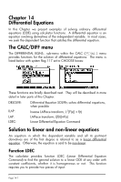
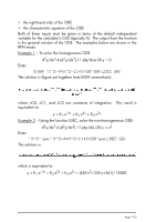
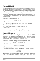
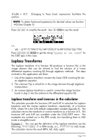
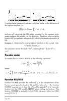
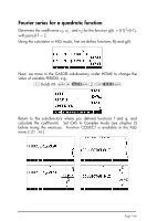
Function DESOLVE The calculator provides function DESOLVE (Differential Equation SOLVEr) to solve certain types of differential equations. The function requires as input the differential equation and the unknown function, and returns the solution to the equation if available. You can also provide a vector containing the differential equation and the initial conditions, instead of only a differential equation, as input to DESOLVE. The function DESOLVE is available in the CALC/DIFF menu. Examples of DESOLVE applications are shown below using RPN mode. Example 1 - Solve the first-order ODE: dy/dx + x2⋅y(x) = 5. In the calculator use: 'd1y(x)+x^2*y(x)=5' ` 'y(x)' ` DESOLVE The solution provided is {'y(x) = (5*INT(EXP(xt^3/3),xt,x)+cC0)*1/EXP(x^3/3)}' } , which simplifies to ( ) y(x) = 5 ⋅ exp(−x 3 / 3) ⋅ ∫ exp(x 3 / 3) ⋅ dx + C0 . The variable ODETYPE You will notice in the soft-menu key labels a new variable called @ODETY (ODETYPE). This variable is produced with the call to the DESOL function and holds a string showing the type of ODE used as input for DESOLVE. Press @ODETY to obtain the string "1st order linear". Example 2 - Solving an equation with initial conditions. Solve d2y/dt2 + 5y = 2 cos(t/2), with initial conditions y(0) = 1.2, y'(0) = -0.5. In the calculator, use: ['d1d1y(t)+5*y(t) = 2*COS(t/2)' 'y(0) = 6/5' 'd1y(0) = -1/2'] ` 'y(t)' ` DESOLVE Notice that the initial conditions were changed to their Exact expressions, 'y(0) = 6/5', rather than 'y(0)=1.2', and 'd1y(0) = -1/2', rather than, Page 14-3