HP 40gs HP 39gs_40gs_Mastering The Graphing Calculator_English_E_F2224-90010.p - Page 142
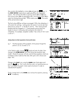
The lower horizontal line shows the, equivalent critical sample mean range.
 |
UPC - 882780045217
View all HP 40gs manuals
Add to My Manuals
Save this manual to your list of manuals |
Page 142 highlights
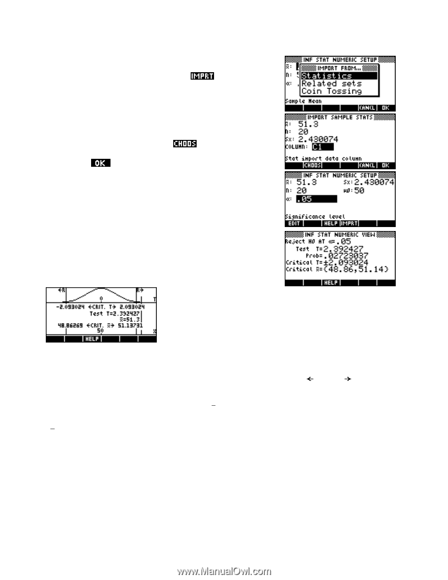
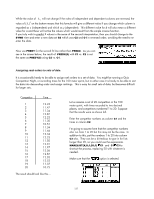
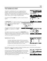
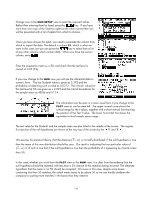
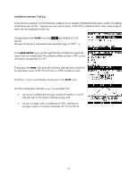
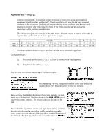
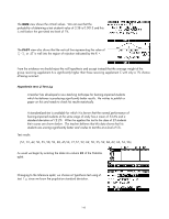
Change now to the NUM SETUP view to enter the required values. Rather than entering them by hand, press the key. If you have more than one copy of the Statistics aplet (under other names) then you will be presented with a list of aplets from which to choose. Once you have chosen the aplet, you need to nominate the column from which to import the data. The default is column C1, which is what we want in this case, but you can press the key to select from a list of any other columns which contain data. When you have the correct column, press . Enter the population mean µ0 = 50, and check that the test level is correct at 0.05 (5%). If you now change to the NUM view you will see the inferential data in numeric form. The test Student-t value is given as 2.392 and the probability of obtaining such a value as 0.0272. The critical t values for this test level of 5% are given as ± 2.093 and the critical boundaries for the sample mean as 48.86 and 51.14. The information can be seen in a more visual form if you change to the PLOT view as can be seen left. The upper normal curve shows the critical range for the t values, together with a short vertical line showing the position of the Test T value. The lower horizontal line shows the equivalent critical sample mean range. The test value for the Student-t and the sample mean are also listed in the middle of the screen. The regions for rejection of the null hypotheses are shown at the very top of the screen by the ' R' and 'R '. ( ) We assume, by statistical theory, that the distance x − µ is normally distributed. If the null hypothesis is true then the mean of this new distribution should be zero. Our result is indicating that our particular value of ( ) x − µ is of such a size that if the null hypothesis is true then the probability of it appearing by chance is less than 5%. In this case, whether you work from the PLOT view or the NUM view, it is clear from the evidence that the null hypothesis should be rejected, with less than a 5% chance of this rejection being incorrect. The alternate hypothesis that the mean is not 50 should be accepted. Of course in this case, despite some boxes containing less than 50 matches, the actual mean seems to be above 50 so we can hardly condemn the company for putting more matches in the boxes than they need to! 142
-
 1
1 -
2
-
3
-
4
-
5
-
6
-
7
-
8
-
9
-
10
-
11
-
12
-
13
-
14
-
15
-
16
-
17
-
18
-
19
-
20
-
21
-
22
-
23
-
24
-
25
-
26
-
27
-
28
-
29
-
30
-
31
-
32
-
33
-
34
-
35
-
36
-
37
-
38
-
39
-
40
-
41
-
42
-
43
-
44
-
45
-
46
-
47
-
48
-
49
-
50
-
51
-
52
-
53
-
54
-
55
-
56
-
57
-
58
-
59
-
60
-
61
-
62
-
63
-
64
-
65
-
66
-
67
-
68
-
69
-
70
-
71
-
72
-
73
-
74
-
75
-
76
-
77
-
78
-
79
-
80
-
81
-
82
-
83
-
84
-
85
-
86
-
87
-
88
-
89
-
90
-
91
-
92
-
93
-
94
-
95
-
96
-
97
-
98
-
99
-
100
-
101
-
102
-
103
-
104
-
105
-
106
-
107
-
108
-
109
-
110
-
111
-
112
-
113
-
114
-
115
-
116
-
117
-
118
-
119
-
120
-
121
-
122
-
123
-
124
-
125
-
126
-
127
-
128
-
129
-
130
-
131
-
132
-
133
-
134
-
135
-
136
-
 137
137 -
 138
138 -
 139
139 -
 140
140 -
 141
141 -
 142
142 -
 143
143 -
 144
144 -
 145
145 -
 146
146 -
 147
147 -
148
-
149
-
150
-
151
-
152
-
153
-
154
-
155
-
156
-
157
-
158
-
159
-
160
-
161
-
162
-
163
-
164
-
165
-
166
-
167
-
168
-
169
-
170
-
171
-
172
-
173
-
174
-
175
-
176
-
177
-
178
-
179
-
180
-
181
-
182
-
183
-
184
-
185
-
186
-
187
-
188
-
189
-
190
-
191
-
192
-
193
-
194
-
195
-
196
-
197
-
198
-
199
-
200
-
201
-
202
-
203
-
204
-
205
-
206
-
207
-
208
-
209
-
210
-
211
-
212
-
213
-
214
-
215
-
216
-
217
-
218
-
219
-
220
-
221
-
222
-
223
-
224
-
225
-
226
-
227
-
228
-
229
-
230
-
231
-
232
-
233
-
234
-
235
-
236
-
237
-
238
-
239
-
240
-
241
-
242
-
243
-
244
-
245
-
246
-
247
-
248
-
249
-
250
-
251
-
252
-
253
-
254
-
255
-
256
-
257
-
258
-
259
-
260
-
261
-
262
-
263
-
264
-
265
-
266
-
267
-
268
-
269
-
270
-
271
-
272
-
273
-
274
-
275
-
276
-
277
-
278
-
279
-
280
-
281
-
282
-
283
-
284
-
285
-
286
-
287
-
288
-
289
-
290
-
291
-
292
-
293
-
294
-
295
-
296
-
297
-
298
-
299
-
300
-
301
-
302
-
303
-
304
-
305
-
306
-
307
-
308
-
309
-
310
-
311
-
312
-
313
-
314
-
315
-
316
-
317
-
318
-
319
-
320
-
321
-
322
-
323
-
324
-
325
-
326
-
327
-
328
-
329
-
330
-
331
-
332
-
333
-
334
-
335
-
336
-
337
-
338
-
339
-
340
-
341
-
342
-
343
-
344
-
345
-
346
-
347
-
348
-
349
-
350
-
351
-
352
-
353
-
354
-
355
-
356
-
357
-
358
-
359
-
360
-
361
-
362
-
363
-
364
-
365
-
366
 |
 |