Texas Instruments TINSPIRE Teacher Software Guidebook - Page 587
Linear Regression mx+b LinRegMx - cx calculator
 |
View all Texas Instruments TINSPIRE manuals
Add to My Manuals
Save this manual to your list of manuals |
Page 587 highlights
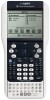
• correlation coefficient, R. Linear Regression (mx+b) (LinRegMx) fits the model equation y=ax+b to the data using a least-squares fit. It displays values for m (slope) and b (y-intercept). Linear Regression (a+bx) (LinRegBx) fits the model equation y=a+bx to the data using a least-squares fit. It displays values for a (y-intercept), b (slope), r2, and r. Median-Median Line (MedMed) fits the model equation y=mx+b to the data using the median-median line (resistant line) technique, calculating the summary points x1, y1, x2, y2, x3, and y3. Median-Median Line displays values for m (slope) and b (y-intercept). Quadratic Regression (QuadReg) fits the second-degree polynomial y=ax2+bx+c to the data. It displays values for a, b, c, and R2. For three data points, the equation is a polynomial fit; for four or more, it is a polynomial regression. At least three data points are required. Cubic Regression (CubicReg) fits the third-degree polynomial y=ax3+bx2+cx+d to the data. It displays values for a, b, c, d, and R2. For four points, the equation is a polynomial fit; for five or more, it is a polynomial regression. At least four points are required. Quartic Regression (QuartReg) fits the fourth-degree polynomial y=ax4+bx3+cx2+dx+e to the data. It displays values for a, b, c, d, e, and R2. For five points, the equation is a polynomial fit; for six or more, it is a polynomial regression. At least five points are required. Power Regression (PowerReg) fits the model equation y=axb to the data using a least-squares fit on transformed values ln(x) and ln(y). It displays values for a, b, r2, and r. Exponential Regression (ExpReg) fits the model equation y=abx to the data using a least-squares fit on transformed values x and ln(y). It displays values for a, b, r2, and r. Logarithmic Regression (LogReg) fits the model equation y=a+b ln(x) to the data using a least-squares fit on transformed values ln(x) and y. It displays values for a, b, r2, and r. Sinusoidal Regression (SinReg) fits the model equation y=a sin(bx+c)+d to the data using an iterative least-squares fit. It displays values for a, b, c, and d. At least four data points are required. At least two data points per cycle are required in order to avoid aliased frequency estimates. Using Lists & Spreadsheet 575
-
 1
1 -
2
-
3
-
4
-
5
-
6
-
7
-
8
-
9
-
10
-
11
-
12
-
13
-
14
-
15
-
16
-
17
-
18
-
19
-
20
-
21
-
22
-
23
-
24
-
25
-
26
-
27
-
28
-
29
-
30
-
31
-
32
-
33
-
34
-
35
-
36
-
37
-
38
-
39
-
40
-
41
-
42
-
43
-
44
-
45
-
46
-
47
-
48
-
49
-
50
-
51
-
52
-
53
-
54
-
55
-
56
-
57
-
58
-
59
-
60
-
61
-
62
-
63
-
64
-
65
-
66
-
67
-
68
-
69
-
70
-
71
-
72
-
73
-
74
-
75
-
76
-
77
-
78
-
79
-
80
-
81
-
82
-
83
-
84
-
85
-
86
-
87
-
88
-
89
-
90
-
91
-
92
-
93
-
94
-
95
-
96
-
97
-
98
-
99
-
100
-
101
-
102
-
103
-
104
-
105
-
106
-
107
-
108
-
109
-
110
-
111
-
112
-
113
-
114
-
115
-
116
-
117
-
118
-
119
-
120
-
121
-
122
-
123
-
124
-
125
-
126
-
127
-
128
-
129
-
130
-
131
-
132
-
133
-
134
-
135
-
136
-
137
-
138
-
139
-
140
-
141
-
142
-
143
-
144
-
145
-
146
-
147
-
148
-
149
-
150
-
151
-
152
-
153
-
154
-
155
-
156
-
157
-
158
-
159
-
160
-
161
-
162
-
163
-
164
-
165
-
166
-
167
-
168
-
169
-
170
-
171
-
172
-
173
-
174
-
175
-
176
-
177
-
178
-
179
-
180
-
181
-
182
-
183
-
184
-
185
-
186
-
187
-
188
-
189
-
190
-
191
-
192
-
193
-
194
-
195
-
196
-
197
-
198
-
199
-
200
-
201
-
202
-
203
-
204
-
205
-
206
-
207
-
208
-
209
-
210
-
211
-
212
-
213
-
214
-
215
-
216
-
217
-
218
-
219
-
220
-
221
-
222
-
223
-
224
-
225
-
226
-
227
-
228
-
229
-
230
-
231
-
232
-
233
-
234
-
235
-
236
-
237
-
238
-
239
-
240
-
241
-
242
-
243
-
244
-
245
-
246
-
247
-
248
-
249
-
250
-
251
-
252
-
253
-
254
-
255
-
256
-
257
-
258
-
259
-
260
-
261
-
262
-
263
-
264
-
265
-
266
-
267
-
268
-
269
-
270
-
271
-
272
-
273
-
274
-
275
-
276
-
277
-
278
-
279
-
280
-
281
-
282
-
283
-
284
-
285
-
286
-
287
-
288
-
289
-
290
-
291
-
292
-
293
-
294
-
295
-
296
-
297
-
298
-
299
-
300
-
301
-
302
-
303
-
304
-
305
-
306
-
307
-
308
-
309
-
310
-
311
-
312
-
313
-
314
-
315
-
316
-
317
-
318
-
319
-
320
-
321
-
322
-
323
-
324
-
325
-
326
-
327
-
328
-
329
-
330
-
331
-
332
-
333
-
334
-
335
-
336
-
337
-
338
-
339
-
340
-
341
-
342
-
343
-
344
-
345
-
346
-
347
-
348
-
349
-
350
-
351
-
352
-
353
-
354
-
355
-
356
-
357
-
358
-
359
-
360
-
361
-
362
-
363
-
364
-
365
-
366
-
367
-
368
-
369
-
370
-
371
-
372
-
373
-
374
-
375
-
376
-
377
-
378
-
379
-
380
-
381
-
382
-
383
-
384
-
385
-
386
-
387
-
388
-
389
-
390
-
391
-
392
-
393
-
394
-
395
-
396
-
397
-
398
-
399
-
400
-
401
-
402
-
403
-
404
-
405
-
406
-
407
-
408
-
409
-
410
-
411
-
412
-
413
-
414
-
415
-
416
-
417
-
418
-
419
-
420
-
421
-
422
-
423
-
424
-
425
-
426
-
427
-
428
-
429
-
430
-
431
-
432
-
433
-
434
-
435
-
436
-
437
-
438
-
439
-
440
-
441
-
442
-
443
-
444
-
445
-
446
-
447
-
448
-
449
-
450
-
451
-
452
-
453
-
454
-
455
-
456
-
457
-
458
-
459
-
460
-
461
-
462
-
463
-
464
-
465
-
466
-
467
-
468
-
469
-
470
-
471
-
472
-
473
-
474
-
475
-
476
-
477
-
478
-
479
-
480
-
481
-
482
-
483
-
484
-
485
-
486
-
487
-
488
-
489
-
490
-
491
-
492
-
493
-
494
-
495
-
496
-
497
-
498
-
499
-
500
-
501
-
502
-
503
-
504
-
505
-
506
-
507
-
508
-
509
-
510
-
511
-
512
-
513
-
514
-
515
-
516
-
517
-
518
-
519
-
520
-
521
-
522
-
523
-
524
-
525
-
526
-
527
-
528
-
529
-
530
-
531
-
532
-
533
-
534
-
535
-
536
-
537
-
538
-
539
-
540
-
541
-
542
-
543
-
544
-
545
-
546
-
547
-
548
-
549
-
550
-
551
-
552
-
553
-
554
-
555
-
556
-
557
-
558
-
559
-
560
-
561
-
562
-
563
-
564
-
565
-
566
-
567
-
568
-
569
-
570
-
571
-
572
-
573
-
574
-
575
-
576
-
577
-
578
-
579
-
580
-
581
-
 582
582 -
 583
583 -
 584
584 -
 585
585 -
 586
586 -
 587
587 -
 588
588 -
 589
589 -
 590
590 -
 591
591 -
 592
592 -
593
-
594
-
595
-
596
-
597
-
598
-
599
-
600
-
601
-
602
-
603
-
604
-
605
-
606
-
607
-
608
-
609
-
610
-
611
-
612
-
613
-
614
-
615
-
616
-
617
-
618
-
619
-
620
-
621
-
622
-
623
-
624
-
625
-
626
-
627
-
628
-
629
-
630
-
631
-
632
-
633
-
634
-
635
-
636
-
637
-
638
-
639
-
640
-
641
-
642
-
643
-
644
-
645
-
646
-
647
-
648
-
649
-
650
-
651
-
652
-
653
-
654
-
655
-
656
-
657
-
658
-
659
-
660
-
661
-
662
-
663
-
664
-
665
-
666
-
667
-
668
-
669
-
670
-
671
-
672
-
673
-
674
-
675
-
676
-
677
-
678
-
679
-
680
-
681
-
682
-
683
-
684
-
685
-
686
-
687
-
688
-
689
-
690
-
691
-
692
-
693
-
694
-
695
-
696
-
697
-
698
-
699
-
700
-
701
-
702
-
703
-
704
-
705
-
706
-
707
-
708
-
709
-
710
-
711
-
712
-
713
-
714
-
715
-
716
-
717
-
718
-
719
-
720
-
721
-
722
-
723
-
724
-
725
-
726
-
727
-
728
-
729
-
730
-
731
-
732
-
733
-
734
-
735
-
736
-
737
-
738
-
739
-
740
-
741
-
742
-
743
-
744
-
745
-
746
-
747
-
748
-
749
-
750
-
751
-
752
-
753
-
754
-
755
-
756
-
757
-
758
-
759
-
760
-
761
-
762
-
763
-
764
-
765
-
766
-
767
-
768
-
769
-
770
-
771
-
772
-
773
-
774
-
775
-
776
-
777
-
778
-
779
-
780
-
781
-
782
-
783
-
784
-
785
-
786
-
787
-
788
-
789
-
790
-
791
-
792
-
793
-
794
-
795
-
796
-
797
-
798
-
799
-
800
-
801
-
802
-
803
-
804
-
805
-
806
-
807
-
808
-
809
-
810
-
811
-
812
-
813
-
814
-
815
-
816
-
817
-
818
-
819
-
820
-
821
-
822
-
823
-
824
-
825
-
826
-
827
-
828
-
829
-
830
-
831
-
832
-
833
-
834
-
835
-
836
-
837
-
838
-
839
-
840
-
841
-
842
-
843
-
844
-
845
-
846
-
847
-
848
-
849
-
850
-
851
-
852
-
853
-
854
-
855
-
856
-
857
-
858
-
859
-
860
-
861
-
862
-
863
-
864
-
865
-
866
-
867
-
868
-
869
-
870
-
871
-
872
-
873
-
874
-
875
-
876
 |
 |
