HP 35s HP 35s scientific calculator - User Guide - Page 323
More about Solving, How SOLVE Finds a Root
 |
UPC - 000000000000
View all HP 35s manuals
Add to My Manuals
Save this manual to your list of manuals |
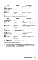
Page 323 highlights
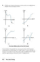
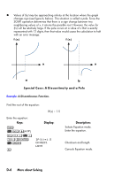
D More about Solving This appendix provides information about the SOLVE operation beyond that given in chapter 7. How SOLVE Finds a Root SOLVE first attempts to solve the equation directly for the unknown variable. If the attempt fails, SOLVE changes to an iterative(repetitive) procedure. The iterative operation is to execute repetitively the specified equation. The value returned by the equation is a function f(x) of the unknown variable x. (f(x) is mathematical shorthand for a function defined in terms of the unknown variable x.) SOLVE starts with an estimate for the unknown variable, x, and refines that estimate with each successive execution of the function, f(x). If any two successive estimates of the function f(x) have opposite signs, then SOLVE presumes that the function f(x) crosses the x-axis in at least one place between the two estimates. This interval is systematically narrowed until a root is found. For SOLVE to find a root, the root has to exist within the range of numbers of the calculator, and the function must be mathematically defined where the iterative search occurs. SOLVE always finds a root, provided one exists (within the overflow bounds), if one or more of these conditions are met: Two estimates yield f(x) values with opposite signs, and the function's graph crosses the x-axis in at least one place between those estimates (figure a, below). f(x) always increases or always decreases as x increases (figure b, below). The graph of f(x) is either concave everywhere or convex everywhere (figure c, below). More about Solving D-1
-
 1
1 -
2
-
3
-
4
-
5
-
6
-
7
-
8
-
9
-
10
-
11
-
12
-
13
-
14
-
15
-
16
-
17
-
18
-
19
-
20
-
21
-
22
-
23
-
24
-
25
-
26
-
27
-
28
-
29
-
30
-
31
-
32
-
33
-
34
-
35
-
36
-
37
-
38
-
39
-
40
-
41
-
42
-
43
-
44
-
45
-
46
-
47
-
48
-
49
-
50
-
51
-
52
-
53
-
54
-
55
-
56
-
57
-
58
-
59
-
60
-
61
-
62
-
63
-
64
-
65
-
66
-
67
-
68
-
69
-
70
-
71
-
72
-
73
-
74
-
75
-
76
-
77
-
78
-
79
-
80
-
81
-
82
-
83
-
84
-
85
-
86
-
87
-
88
-
89
-
90
-
91
-
92
-
93
-
94
-
95
-
96
-
97
-
98
-
99
-
100
-
101
-
102
-
103
-
104
-
105
-
106
-
107
-
108
-
109
-
110
-
111
-
112
-
113
-
114
-
115
-
116
-
117
-
118
-
119
-
120
-
121
-
122
-
123
-
124
-
125
-
126
-
127
-
128
-
129
-
130
-
131
-
132
-
133
-
134
-
135
-
136
-
137
-
138
-
139
-
140
-
141
-
142
-
143
-
144
-
145
-
146
-
147
-
148
-
149
-
150
-
151
-
152
-
153
-
154
-
155
-
156
-
157
-
158
-
159
-
160
-
161
-
162
-
163
-
164
-
165
-
166
-
167
-
168
-
169
-
170
-
171
-
172
-
173
-
174
-
175
-
176
-
177
-
178
-
179
-
180
-
181
-
182
-
183
-
184
-
185
-
186
-
187
-
188
-
189
-
190
-
191
-
192
-
193
-
194
-
195
-
196
-
197
-
198
-
199
-
200
-
201
-
202
-
203
-
204
-
205
-
206
-
207
-
208
-
209
-
210
-
211
-
212
-
213
-
214
-
215
-
216
-
217
-
218
-
219
-
220
-
221
-
222
-
223
-
224
-
225
-
226
-
227
-
228
-
229
-
230
-
231
-
232
-
233
-
234
-
235
-
236
-
237
-
238
-
239
-
240
-
241
-
242
-
243
-
244
-
245
-
246
-
247
-
248
-
249
-
250
-
251
-
252
-
253
-
254
-
255
-
256
-
257
-
258
-
259
-
260
-
261
-
262
-
263
-
264
-
265
-
266
-
267
-
268
-
269
-
270
-
271
-
272
-
273
-
274
-
275
-
276
-
277
-
278
-
279
-
280
-
281
-
282
-
283
-
284
-
285
-
286
-
287
-
288
-
289
-
290
-
291
-
292
-
293
-
294
-
295
-
296
-
297
-
298
-
299
-
300
-
301
-
302
-
303
-
304
-
305
-
306
-
307
-
308
-
309
-
310
-
311
-
312
-
313
-
314
-
315
-
316
-
317
-
 318
318 -
 319
319 -
 320
320 -
 321
321 -
 322
322 -
 323
323 -
 324
324 -
 325
325 -
 326
326 -
 327
327 -
 328
328 -
329
-
330
-
331
-
332
-
333
-
334
-
335
-
336
-
337
-
338
-
339
-
340
-
341
-
342
-
343
-
344
-
345
-
346
-
347
-
348
-
349
-
350
-
351
-
352
-
353
-
354
-
355
-
356
-
357
-
358
-
359
-
360
-
361
-
362
-
363
-
364
-
365
-
366
-
367
-
368
-
369
-
370
-
371
-
372
-
373
-
374
-
375
-
376
-
377
-
378
-
379
-
380
-
381
-
382
 |
 |