HP HP12C hp 12c_user's guide_English_E_HDPMBF12E44.pdf - Page 148

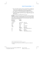
148 Section 13: Investment Analysis Excess Depreciation When accelerated depreciation is used, the difference between total depreciation charged over a given period of time and the total amount that would have been charged under straight-line depreciation is called excess depreciation. To obtain excess depreciation: 1. Calculate the total depreciation then press \. 2. Key in the depreciable amount (cost less salvage) then press \. Key in the useful life of the asset in years then press z. Key in the number of years in the income projection period then press § to get the total straight-line depreciation charge. 3. Press - to get the excess depreciation. Example: What is the excess depreciation in the previous example over 7 calendar years? (Because of the partial first year, there are 61/2 years depreciation in the first 7 calendar years.) Keystrokes 9429.56\ 10500\ 8z 6.5§ - Display 9,429.56 10,500.00 1,312.50 8,531.25 898.31 Total depreciation through seventh year. Depreciable amount. Yearly straight-line depreciation. Total straight-line depreciation. Excess depreciation Modified Internal Rate of Return The traditional Internal Rate of Return (IRR) technique has several drawbacks which hamper its usefulness in some investment applications. The technique implicitly assumes that all cash flows are either reinvested or discounted at the computed yield rate. This assumption is financially reasonable as long as the rate is within a realistic borrowing and lending range (for example, 10% to 20%). When the IRR becomes significantly greater or smaller, the assumption becomes less valid and the resulting value less sound as an investment measure. IRR also is limited by the number of times the sign of the cash flow changes (positive to negative or vice versa). For every change of sign, the IRR solution has the potential for an additional answer. The cash flow sequence in the example that follows has three sign changes and hence up to three potential internal rates of return. This particular example has three positive real answers: 1.86, 14.35, and 29. Although mathematically sound, multiple answers probably are meaningless as an investment measure. File name: hp 12c_user's guide_English_HDPMBF12E44 Printered Date: 2005/7/29 Page: 148 of 209 Dimension: 14.8 cm x 21 cm