Brother International WP335B Owners Manual - English - Page 218

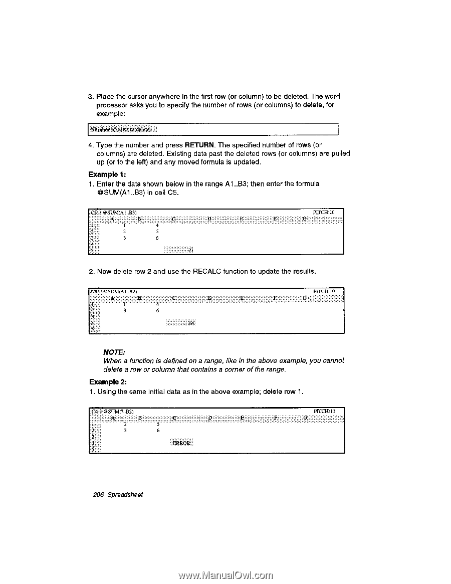
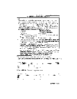
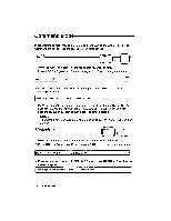
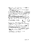
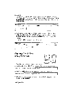
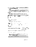
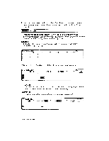
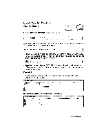
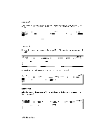
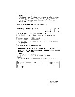
3.

Place

the

cursor

anywhere

in

the

first

row

(or

column)

to

be

deleted.

The

word

processor

asks

you

to

specify

the

number

of

rows

(or

columns)

to

delete,

for

example:

4.

Type

the

number

and

press

RETURN.

The

specified

number

of

rows

(or

columns)

are

deleted.

Existing

data

past

the

deleted

rows

(or

columns)

are

pulled

up

(or

to

the

left)

and

any

moved

formula

is

updated.

Example

1:

1.

Enter

the

data

shown

below

in

the

range

Al

..B3;

then

enter

the

formula

OSUM(A1..B3)

in

cell

C5.

@SLTM(A1..B3)

•

2

2

5

3

6

PITCH:10

2.

Now

delete

row

2

and

use

the

RECALC

function

to

update

the

results.

@SUM(A

1..132)

3

PITCH:10

NOTE:

When

a

function

is

defined

on

a

range,

like

in

the

above

example,

you

cannot

delete

a

row

or

column

that

contains

a

corner

of

the

range.

Example

2:

1.

Using

the

same

initial

data

as

in

the

above

example;

delete

row

1.

SUM(?..B2)

3

PITCH:10

.....

206

Spreadsheet

Brother International WP335B Owners Manual - English - Page 218

Osuma1..b3

Page 218 highlights