Campbell Scientific CSAT3B CSAT3B Three-Dimensional Sonic Anemometer - Page 77
Appendix B. CSAT3B Measurement, Theory
 |
View all Campbell Scientific CSAT3B manuals
Add to My Manuals
Save this manual to your list of manuals |
Page 77 highlights
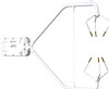
Appendix B. CSAT3B Measurement Theory B.1 Theory of Operation B.1.1 Wind Speed Each axis of the CSAT3B pulses two ultrasonic signals in opposite directions. The time of flight of the first signal (out) is given by: d to = c + ua (B-1) and the time of flight of the second signal (back) is given by: d tb = c - ua (B-2) where: to = time of flight out along the transducer axis tb = time of flight back, in the opposite direction ua = wind speed along the transducer axis d = distance between the transducers c = speed of sound The wind speed, ua, along any axis can be found by inverting the above relationships, then subtracting Eq. (B-2) from (B-1) and solving for ua. d 1 1 ua = 2 to − tb (B-3) The wind speed is measured on all three non-orthogonal axis to give ua, ub, and uc, where the subscripts a, b, and c refer to the non-orthogonal sonic axis. The non-orthogonal wind speed components are then transformed into orthogonal wind speed components, ux, uy, and uz, with the following: u x ua uy = Aub uz uc (B-4) where: A = a 3 x 3 coordinate transformation matrix, that is unique for each CSAT3B and is stored in ROM memory B-1
-
 1
1 -
2
-
3
-
4
-
5
-
6
-
7
-
8
-
9
-
10
-
11
-
12
-
13
-
14
-
15
-
16
-
17
-
18
-
19
-
20
-
21
-
22
-
23
-
24
-
25
-
26
-
27
-
28
-
29
-
30
-
31
-
32
-
33
-
34
-
35
-
36
-
37
-
38
-
39
-
40
-
41
-
42
-
43
-
44
-
45
-
46
-
47
-
48
-
49
-
50
-
51
-
52
-
53
-
54
-
55
-
56
-
57
-
58
-
59
-
60
-
61
-
62
-
63
-
64
-
65
-
66
-
67
-
68
-
69
-
70
-
71
-
 72
72 -
 73
73 -
 74
74 -
 75
75 -
 76
76 -
 77
77 -
 78
78 -
 79
79 -
 80
80 -
 81
81 -
 82
82 -
83
-
84
-
85
-
86
-
87
-
88
 |
 |
