HP 50g HP 50g_user's manual_English_HDPSG49AEM8.pdf - Page 147

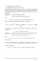
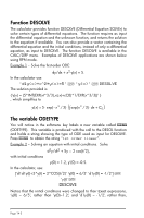
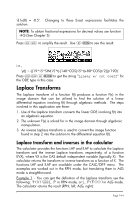
'd1y(0) = -0.5'. Changing to these Exact expressions facilitates the solution. NOTE: To obtain fractional expressions for decimal values use function Q (See Chapter 5). Press µµ to simplify the result. Use ˜ @EDIT to see this result: i.e., 'y(t) = -((19*√5*SIN(√5*t)-(148*COS(√5*t)+80*COS(t/2)))/190)'. Press ``J@ODETY to get the string "Linear w/ cst coeff" for the ODE type in this case. Laplace Transforms The Laplace transform of a function f(t) produces a function F(s) in the image domain that can be utilized to find the solution of a linear differential equation involving f(t) through algebraic methods. The steps involved in this application are three: 1. Use of the Laplace transform converts the linear ODE involving f(t) into an algebraic equation. 2. The unknown F(s) is solved for in the image domain through algebraic manipulation. 3. An inverse Laplace transform is used to convert the image function found in step 2 into the solution to the differential equation f(t). Laplace transform and inverses in the calculator The calculator provides the functions LAP and ILAP to calculate the Laplace transform and the inverse Laplace transform, respectively, of a function f(VX), where VX is the CAS default independent variable (typically X). The calculator returns the transform or inverse transform as a function of X. The functions LAP and ILAP are available under the CALC/DIFF menu. The examples are worked out in the RPN mode, but translating them to ALG mode is straightforward. Example 1 - You can get the definition of the Laplace transform use the following: 'f(X)'`LAP in RPN mode, or LAP(F(X))in ALG mode. The calculator returns the result (RPN, left; ALG, right): Page 14-4