HP 50g HP 50g_user's manual_English_HDPSG49AEM8.pdf - Page 159
Frequencies.., DAT vector, 14 values smaller than -8
 |
UPC - 882780502291
View all HP 50g manuals
Add to My Manuals
Save this manual to your list of manuals |
Page 159 highlights
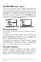
ΣDAT, by using function STOΣ (see example above). Next, obtain singlevariable information using: ,Ù @@@OK@@@. The results are: This information indicates that our data ranges from -9 to 9. To produce a frequency distribution we will use the interval (-8, 8) dividing it into 8 bins of width 2 each. • Select the program 2. Frequencies.. by using ,Ù˜ @@@OK@@@. The data is already loaded in ΣDAT, and the option Col should hold the value 1 since we have only one column in ΣDAT. • Change X-Min to -8, Bin Count to 8, and Bin Width to 2, then press @@@OK@@@. Using the RPN mode, the results are shown in the stack as a column vector in stack level 2, and a row vector of two components in stack level 1. The vector in stack level 1 is the number of outliers outside of the interval where the frequency count was performed. For this case, I get the values [14. 8.] indicating that there are, in the ΣDAT vector, 14 values smaller than -8 and 8 larger than 8. • Press ƒ to drop the vector of outliers from the stack. The remaining result is the frequency count of data. The bins for this frequency distribution will be: -8 to -6, -6 to -4, ..., 4 to 6, and 6 to 8, i.e., 8 of them, with the frequencies in the column vector in the stack, namely (for this case): 23, 22, 22, 17, 26, 15, 20, 33. This means that there are 23 values in the bin [-8,-6], 22 in [-6,-4], 22 in [4,-2], 17 in [-2,0], 26 in [0,2], 15 in [2,4], 20 in [4,6], and 33 in [6,8]. You can also check that adding all these values plus the outliers, 14 and 8, show above, you will get the total number of elements in the sample, namely, 200. Page 16-4
-
 1
1 -
2
-
3
-
4
-
5
-
6
-
7
-
8
-
9
-
10
-
11
-
12
-
13
-
14
-
15
-
16
-
17
-
18
-
19
-
20
-
21
-
22
-
23
-
24
-
25
-
26
-
27
-
28
-
29
-
30
-
31
-
32
-
33
-
34
-
35
-
36
-
37
-
38
-
39
-
40
-
41
-
42
-
43
-
44
-
45
-
46
-
47
-
48
-
49
-
50
-
51
-
52
-
53
-
54
-
55
-
56
-
57
-
58
-
59
-
60
-
61
-
62
-
63
-
64
-
65
-
66
-
67
-
68
-
69
-
70
-
71
-
72
-
73
-
74
-
75
-
76
-
77
-
78
-
79
-
80
-
81
-
82
-
83
-
84
-
85
-
86
-
87
-
88
-
89
-
90
-
91
-
92
-
93
-
94
-
95
-
96
-
97
-
98
-
99
-
100
-
101
-
102
-
103
-
104
-
105
-
106
-
107
-
108
-
109
-
110
-
111
-
112
-
113
-
114
-
115
-
116
-
117
-
118
-
119
-
120
-
121
-
122
-
123
-
124
-
125
-
126
-
127
-
128
-
129
-
130
-
131
-
132
-
133
-
134
-
135
-
136
-
137
-
138
-
139
-
140
-
141
-
142
-
143
-
144
-
145
-
146
-
147
-
148
-
149
-
150
-
151
-
152
-
153
-
 154
154 -
 155
155 -
 156
156 -
 157
157 -
 158
158 -
 159
159 -
 160
160 -
 161
161 -
 162
162 -
 163
163 -
 164
164 -
165
-
166
-
167
-
168
-
169
-
170
-
171
-
172
-
173
-
174
-
175
-
176
-
177
-
178
-
179
-
180
-
181
-
182
-
183
-
184
 |
 |
