Texas Instruments TI-73VSC Guidebook - Page 120

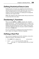
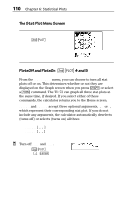
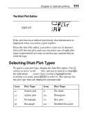
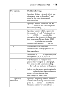
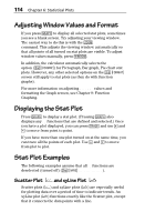
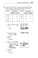
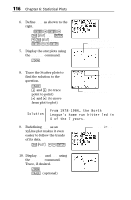
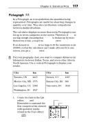
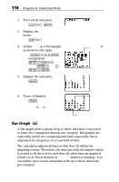
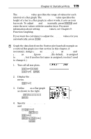
114 Chapter 6: Statistical Plots Adjusting Window Values and Format If you press * to display all selected stat plots, sometimes you see a blank screen. Try adjusting your viewing window. The easiest way to do this is with the ( 7:ZoomStat command. This adjusts the viewing window automatically so that all points of all turned on stat plots are visible. To adjust window values manually, press '. In addition, the calculator automatically selects the AxesOff option (- g) for Pictograph, Bar graph, Pie chart stat plots. However, any other selected options on the - g screen still apply to stat plots (as they do with function graphs). For more information on adjusting WINDOW values and formatting the Graph screen, see Chapter 9: Function Graphing. Displaying the Stat Plot Press * to display a stat plot. (Pressing * also displays any Yn functions that are defined and selected.) Once you have a plot displayed, you can press ) and use " and ! to move from point to point. If you have more than one plot turned on at the same time, you can trace all the points of each plot. Use $ and # to move from plot to plot. Stat Plot Examples The following examples assume that all Yn functions are deselected (turned off) (- } 2:Y-Vars 6:FnOff). Scatter Plot Ô and xyLine Plot Ó Scatter plots (Ô) and xyLine plots (Ó) are especially useful for plotting data over a period of time to indicate trends. An xyLine plot (Ó) functions exactly like the Scatter plot, except that it connects the data points with a line.