Texas Instruments TI-84 PLUS SILV Guidebook - Page 189

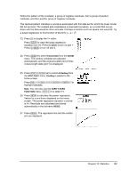
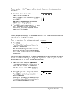
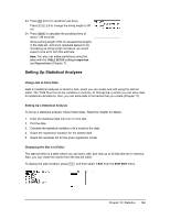
Notice the pattern of the residuals: a group of negative residuals, then a group of positive residuals, and then another group of negative residuals. The residual pattern indicates a curvature associated with this data set for which the linear model did not account. The residual plot emphasizes a downward curvature, so a model that curves down with the data would be more accurate. Perhaps a function such as square root would fit. Try a power regression to fit a function of the form y = a ... xb. 23. Press o to display the Y= editor. Press ' to clear the linear regression equation from Y1. Press } Í to turn on plot 1. Press ~ Í to turn off plot 2. 24. Press q 9 to select 9:ZoomStat from the ZOOM menu. The window variables are adjusted automatically, and the original scatter plot of timeversus-length data (plot 1) is displayed. 25. Press ... ~ ƒ ãAä to select A:PwrReg from the STAT CALC menu. PwrReg is pasted to the home screen. Press y d † y e † † t a Í † to highlight Calculate. Note: You can also use the VARS Y-VARS FUNCTION menu,  ~ 1 to select Y1. 26. Press Í to calculate the power regression. Values for a and b are displayed on the home screen. The power regression equation is stored in Y1. Residuals are calculated and stored automatically in the list name RESID. 27. Press s. The regression line and the scatter plot are displayed. Chapter 12: Statistics 182