Texas Instruments TI-84 PLUS SILV Guidebook - Page 190

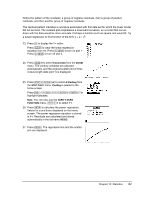
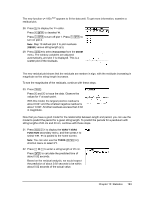
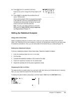
The new function y=.192x.522 appears to fit the data well. To get more information, examine a residual plot. 28. Press o to display the Y= editor. Press | Í to deselect Y1. Press } Í to turn off plot 1. Press ~ Í to turn on plot 2. Note: Step 19 defined plot 2 to plot residuals (RESID) versus string length (L1). 29. Press q 9 to select 9:ZoomStat from the ZOOM menu. The window variables are adjusted automatically, and plot 2 is displayed. This is a scatter plot of the residuals. The new residual plot shows that the residuals are random in sign, with the residuals increasing in magnitude as the string length increases. To see the magnitudes of the residuals, continue with these steps. 30. Press r. Press ~ and | to trace the data. Observe the values for Y at each point. With this model, the largest positive residual is about 0.041 and the smallest negative residual is about L0.027. All other residuals are less than 0.02 in magnitude. Now that you have a good model for the relationship between length and period, you can use the model to predict the period for a given string length. To predict the periods for a pendulum with string lengths of 20 cm and 50 cm, continue with these steps. 31. Press  ~ 1 to display the VARS Y-VARS FUNCTION secondary menu, and then press 1 to select 1:Y1. Y1 is pasted to the home screen. Note: You can also use the YVARS (t a) shortcut menu to select Y1. 32. Press £ 20 ¤ to enter a string length of 20 cm. Press Í to calculate the predicted time of about 0.92 seconds. Based on the residual analysis, we would expect the prediction of about 0.92 seconds to be within about 0.02 seconds of the actual value. Chapter 12: Statistics 183