Texas Instruments TI-84 PLUS SILV Guidebook - Page 212
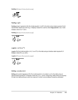
Manual Linear Fit, SinReg, SinReg 16, D:Manual-Fit.
 |
View all Texas Instruments TI-84 PLUS SILV manuals
Add to My Manuals
Save this manual to your list of manuals |
Page 212 highlights
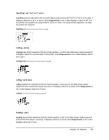
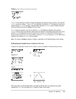
• Plot the data and trace to determine the x-distance between the beginning and end of one complete period, or cycle. The illustration above and to the right graphically depicts a complete period, or cycle. • Plot the data and trace to determine the x-distance between the beginning and end of N complete periods, or cycles. Then divide the total distance by N. After your first attempt to use SinReg and the default value for iterations to fit the data, you may find the fit to be approximately correct, but not optimal. For an optimal fit, execute SinReg 16,Xlistname,Ylistname,2p/b where b is the value obtained from the previous SinReg execution. Manual Linear Fit Manual Linear Fit allows you to visually fit a linear function to a scatter plot. Manual Linear Fit is an option in the ... / menu. After entering List data and viewing the StatPlot, select the Manual-Fit function. 1. Press ... to display the Stat menu. Press ~ to select CALC. Press † several times to scroll down to select D:Manual-Fit. Press Í. This displays a free-floating cursor at the center of the display screen. 2. Press the cursor navigation keys to move the cursor to the desired location. Press Í to select the first point. 3. Press the cursor navigation keys to move the cursor to the second location. Press Í. This displays a line containing the two points selected. The linear function is displayed. The Manual-Fit Line equation displays in the form of Y=mX+b. The current value of the first parameter (m) is highlighted in the symbolic expression. Modify parameter values Press the cursor navigation keys ( | ~ ) to move from the first parameter (m) or (b) the second parameter. You can press Í and type a new parameter value. Press Í to display the new parameter value. When you edit the value of the selected parameter, the edit can include insert, delete, type over, or mathematical expression. The screen dynamically displays the revised parameter value. Press Í to complete the modification of the selected parameter, save the value, and refresh the displayed graph. The Chapter 12: Statistics 205
-
 1
1 -
2
-
3
-
4
-
5
-
6
-
7
-
8
-
9
-
10
-
11
-
12
-
13
-
14
-
15
-
16
-
17
-
18
-
19
-
20
-
21
-
22
-
23
-
24
-
25
-
26
-
27
-
28
-
29
-
30
-
31
-
32
-
33
-
34
-
35
-
36
-
37
-
38
-
39
-
40
-
41
-
42
-
43
-
44
-
45
-
46
-
47
-
48
-
49
-
50
-
51
-
52
-
53
-
54
-
55
-
56
-
57
-
58
-
59
-
60
-
61
-
62
-
63
-
64
-
65
-
66
-
67
-
68
-
69
-
70
-
71
-
72
-
73
-
74
-
75
-
76
-
77
-
78
-
79
-
80
-
81
-
82
-
83
-
84
-
85
-
86
-
87
-
88
-
89
-
90
-
91
-
92
-
93
-
94
-
95
-
96
-
97
-
98
-
99
-
100
-
101
-
102
-
103
-
104
-
105
-
106
-
107
-
108
-
109
-
110
-
111
-
112
-
113
-
114
-
115
-
116
-
117
-
118
-
119
-
120
-
121
-
122
-
123
-
124
-
125
-
126
-
127
-
128
-
129
-
130
-
131
-
132
-
133
-
134
-
135
-
136
-
137
-
138
-
139
-
140
-
141
-
142
-
143
-
144
-
145
-
146
-
147
-
148
-
149
-
150
-
151
-
152
-
153
-
154
-
155
-
156
-
157
-
158
-
159
-
160
-
161
-
162
-
163
-
164
-
165
-
166
-
167
-
168
-
169
-
170
-
171
-
172
-
173
-
174
-
175
-
176
-
177
-
178
-
179
-
180
-
181
-
182
-
183
-
184
-
185
-
186
-
187
-
188
-
189
-
190
-
191
-
192
-
193
-
194
-
195
-
196
-
197
-
198
-
199
-
200
-
201
-
202
-
203
-
204
-
205
-
206
-
 207
207 -
 208
208 -
 209
209 -
 210
210 -
 211
211 -
 212
212 -
 213
213 -
 214
214 -
 215
215 -
 216
216 -
 217
217 -
218
-
219
-
220
-
221
-
222
-
223
-
224
-
225
-
226
-
227
-
228
-
229
-
230
-
231
-
232
-
233
-
234
-
235
-
236
-
237
-
238
-
239
-
240
-
241
-
242
-
243
-
244
-
245
-
246
-
247
-
248
-
249
-
250
-
251
-
252
-
253
-
254
-
255
-
256
-
257
-
258
-
259
-
260
-
261
-
262
-
263
-
264
-
265
-
266
-
267
-
268
-
269
-
270
-
271
-
272
-
273
-
274
-
275
-
276
-
277
-
278
-
279
-
280
-
281
-
282
-
283
-
284
-
285
-
286
-
287
-
288
-
289
-
290
-
291
-
292
-
293
-
294
-
295
-
296
-
297
-
298
-
299
-
300
-
301
-
302
-
303
-
304
-
305
-
306
-
307
-
308
-
309
-
310
-
311
-
312
-
313
-
314
-
315
-
316
-
317
-
318
-
319
-
320
-
321
-
322
-
323
-
324
-
325
-
326
-
327
-
328
-
329
-
330
-
331
-
332
-
333
-
334
-
335
-
336
-
337
-
338
-
339
-
340
-
341
-
342
-
343
-
344
-
345
-
346
-
347
-
348
-
349
-
350
-
351
-
352
-
353
-
354
-
355
-
356
-
357
-
358
-
359
-
360
-
361
-
362
-
363
-
364
-
365
-
366
-
367
-
368
-
369
-
370
-
371
-
372
-
373
-
374
-
375
-
376
-
377
-
378
-
379
-
380
-
381
-
382
-
383
-
384
-
385
-
386
-
387
-
388
-
389
-
390
-
391
-
392
-
393
-
394
-
395
-
396
-
397
-
398
-
399
-
400
-
401
-
402
-
403
-
404
-
405
-
406
-
407
-
408
-
409
-
410
-
411
-
412
-
413
-
414
-
415
-
416
-
417
-
418
-
419
-
420
-
421
-
422
 |
 |
