HP 40gs HP 39gs_40gs_Mastering The Graphing Calculator_English_E_F2224-90010.p - Page 131
Predicting using the PLOT view, RelErr as a measure of non-linear fit
 |
UPC - 882780045217
View all HP 40gs manuals
Add to My Manuals
Save this manual to your list of manuals |
Page 131 highlights
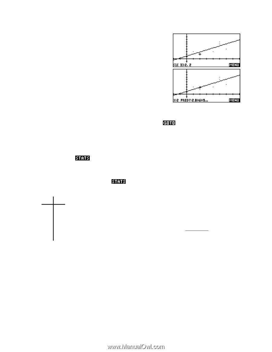
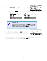
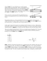
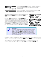
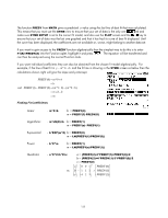
Predicting using the PLOT view Using the PLOT view is the probably the more visually appealing method of obtaining predicted values. When you have plotted a set of data and its fit curve then pressing up arrow will change the focus of the values at the bottom of the screen from the data points to the PREDY values. In the screen snapshots shown right the focus changes from data point 3:(2,2), to the PREDY value for x = 2 of 2.806. If there is more than one data set (and fit lines) graphed then the up arrow will move progressively from one to another and finally back to the first. Pressing left and right arrows will move along the fit line but only on pixel positions, which may not be suitable if the scale is not chosen carefully. A better way is to use the key to obtain PREDY values for any required value of x, including values which would normally be off-screen. Another aspect of bivariate stats needs to be remembered when the fit chosen is not linear. Mathematically, the correlation coefficient is a strictly linear measure of the goodness of fit and this means that the correlation coefficient quoted in the view is always for the linear model even when some other model is chosen. There are two methods of dealing with this. The first is to use another measure of goodness of fit. The second is to 'linearize' the data (discussed on the next page). The calculator provides an alternative measure of goodness of fit via the RelErr value in the view. RelErr as a measure of non-linear fit xi yi 1 2 2 4 3 8 4 16 5 32 6 64 n ∑ ( yi − yˆ)2 RelErr = i=1 n ∑ yi2 i =1 RelErr is defined as the measure of the relative error in predicted values when compared to data values, and has the formula shown right. The smaller the value of RelErr the better the fit. The yˆ values are obtained using the PREDY function internally. The only drawback to RelErr is that there is no upper limit its value of as there is for the correlation coefficient. The interpretation placed on it is that the closer it is to zero the better the model fits the data. This value is available for any of the data models, including the user defined model. 131
-
 1
1 -
2
-
3
-
4
-
5
-
6
-
7
-
8
-
9
-
10
-
11
-
12
-
13
-
14
-
15
-
16
-
17
-
18
-
19
-
20
-
21
-
22
-
23
-
24
-
25
-
26
-
27
-
28
-
29
-
30
-
31
-
32
-
33
-
34
-
35
-
36
-
37
-
38
-
39
-
40
-
41
-
42
-
43
-
44
-
45
-
46
-
47
-
48
-
49
-
50
-
51
-
52
-
53
-
54
-
55
-
56
-
57
-
58
-
59
-
60
-
61
-
62
-
63
-
64
-
65
-
66
-
67
-
68
-
69
-
70
-
71
-
72
-
73
-
74
-
75
-
76
-
77
-
78
-
79
-
80
-
81
-
82
-
83
-
84
-
85
-
86
-
87
-
88
-
89
-
90
-
91
-
92
-
93
-
94
-
95
-
96
-
97
-
98
-
99
-
100
-
101
-
102
-
103
-
104
-
105
-
106
-
107
-
108
-
109
-
110
-
111
-
112
-
113
-
114
-
115
-
116
-
117
-
118
-
119
-
120
-
121
-
122
-
123
-
124
-
125
-
 126
126 -
 127
127 -
 128
128 -
 129
129 -
 130
130 -
 131
131 -
 132
132 -
 133
133 -
 134
134 -
 135
135 -
 136
136 -
137
-
138
-
139
-
140
-
141
-
142
-
143
-
144
-
145
-
146
-
147
-
148
-
149
-
150
-
151
-
152
-
153
-
154
-
155
-
156
-
157
-
158
-
159
-
160
-
161
-
162
-
163
-
164
-
165
-
166
-
167
-
168
-
169
-
170
-
171
-
172
-
173
-
174
-
175
-
176
-
177
-
178
-
179
-
180
-
181
-
182
-
183
-
184
-
185
-
186
-
187
-
188
-
189
-
190
-
191
-
192
-
193
-
194
-
195
-
196
-
197
-
198
-
199
-
200
-
201
-
202
-
203
-
204
-
205
-
206
-
207
-
208
-
209
-
210
-
211
-
212
-
213
-
214
-
215
-
216
-
217
-
218
-
219
-
220
-
221
-
222
-
223
-
224
-
225
-
226
-
227
-
228
-
229
-
230
-
231
-
232
-
233
-
234
-
235
-
236
-
237
-
238
-
239
-
240
-
241
-
242
-
243
-
244
-
245
-
246
-
247
-
248
-
249
-
250
-
251
-
252
-
253
-
254
-
255
-
256
-
257
-
258
-
259
-
260
-
261
-
262
-
263
-
264
-
265
-
266
-
267
-
268
-
269
-
270
-
271
-
272
-
273
-
274
-
275
-
276
-
277
-
278
-
279
-
280
-
281
-
282
-
283
-
284
-
285
-
286
-
287
-
288
-
289
-
290
-
291
-
292
-
293
-
294
-
295
-
296
-
297
-
298
-
299
-
300
-
301
-
302
-
303
-
304
-
305
-
306
-
307
-
308
-
309
-
310
-
311
-
312
-
313
-
314
-
315
-
316
-
317
-
318
-
319
-
320
-
321
-
322
-
323
-
324
-
325
-
326
-
327
-
328
-
329
-
330
-
331
-
332
-
333
-
334
-
335
-
336
-
337
-
338
-
339
-
340
-
341
-
342
-
343
-
344
-
345
-
346
-
347
-
348
-
349
-
350
-
351
-
352
-
353
-
354
-
355
-
356
-
357
-
358
-
359
-
360
-
361
-
362
-
363
-
364
-
365
-
366
 |
 |