HP 40gs HP 39gs_40gs_Mastering The Graphing Calculator_English_E_F2224-90010.p - Page 318

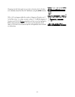
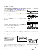
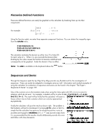
Gradient Function Once the concept of gradient at a point has been established the next step is to develop the idea of a gradient function. This can be done via the Function aplet by using the Slope function which gives the gradient of the graph at the position of the cursor (see page 58). If the teacher has the student enter a function in the SYMB view they can then have the student explore the value of the slope at various values using the the cursor precisely. function to position The Statistics aplet can be used to help with the process of finding gradient functions once tabular data has been collected giving x and slope(x) values. If the student enters the data into C1 and C2, they can then set to , plot the data and make a guess as to the appropriate type of function in the SYMB SETUP view and then use the curve fitting facilities to find an equation. Curves of the form y = mx + b , y = ax2 + bx + c , y = ax3 + bx2 + cx + d and y = axb can be fitted using the ( ) d xn Statistics aplet and this should be enough for the students to deduce the rule = n xn−1 for themselves. It dx is advisable to ensure that the students are familiar with the process of using the Statistics aplet to find equations before commencing, otherwise the two concepts may interfere and confuse. The process can be done in a far more visual style using an aplet downloaded from The HP HOME View web site (http://www.hphomeview.com) called "Tangent Lines". This aplet will add a moveable tangent line to an existing graph, as shown in the screen shot above, allowing the user to move it along the curve with the gradient displayed at the top left of the screen. There are two worksheets included in the documentation which is bundled with this aplet which will take the student through the process of developing a gradient function. 318