Home » HP Manuals » Calculators » HP 40gs » Manual Viewer

HP 40gs HP 39gs_40gs_Mastering The Graphing Calculator_English_E_F2224-90010.p - Page 88

Nice table values, Overlay Plot

UPC - 882780045217

Add to My Manuals
Save this manual to your list of manuals

Page 88 highlights

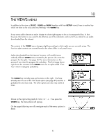
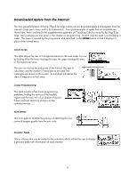
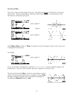
Nice table values What makes this view even more useful is that the table keeps its 'nice' scale even while the usual tools are being used. As you can see in the screenshot left, the table is automatically repositioned to show the closest pixel value to that of the extremum found. The Signed Area tool is also available in this view and when the cursor is moved the values in the table follow it. Unfortunately, the highlighted value in the table doesn't change as the cursor moves to create the shaded area. For this reason the best strategy is to use the key to jump to the end point. This means that the area will not be shaded but this should not be a problem. Overlay Plot Another possibility from the VIEWS menu is Overlay Plot. This option can be used to add another graph over the top of an existing one, without the screen being blanked first as it usually is. As an example, if you have already graphed functions F1(X) through to F6(X) and then add another one in the SYMB view, then you may not want to have to wait while all the earlier ones are redrawn. If you un- the earlier graphs and then use Overlay Plot for the new one then it will be drawn over the top of the existing ones. Of course the results will not be good if the scales don't match!. More usefully, you can use this to combine different styles of graphs. For example, the screen shot right was produced by drawing a circle in the Parametric aplet and then superimposing the equations y = x and y = -x in the Function aplet. This could be used to show, for example, the enclosing curves for conic sections. You can also use this technique to overlay functions on top of statistical graphs. Again, the important point would be to ensure that the scales matched. 88

Section	Page
Title Page	1
Introduction	7
The hp 39gs vs. the hp 40gs	7
Getting Started	9
Some Keyboard Examples	10
Keys & Notation Conventions	11
The SHIFT and ALPHA keys	11
The ALPHA key	11
The Screen keys	12
Pop-up menus & short-cuts	12
Everything revolves around Aplets!	14
The Finance aplet (see page 155)	14
The Function aplet (see page 46)	14
The Inference aplet (see page 141)	14
The Linear Solver aplet (see page 150 )	14
The Parametric aplet (see page 92)	14
The Polar aplet (see page 98)	14
The Quadratic Explorer aplet (see page 159)	14
The Sequence aplet (see page 99)	15
The Solve aplet (see page 105)	15
The Statistics aplet (see page 114 & 123)	15
The Triangle Solve aplet (see page 152 )	15
The Trig Explorer aplet (see page 162)	15
Some typical aplet views	15
The HOME view	18
What is the HOME view?	18
Exploring the keyboard	19
The screen keys	19
Aplet related keys	19
The arrow keys	19
The SYMB, PLOT and NUM keys	20
Intro to the VIEWS menu	21
The VARS key	22
The SETUP views	23
The MODES view	24
Numeric formats	24
The ANS key	26
The negative key	26
The CHARS key	26
The DEL and CLEAR keys	27
Angle and Numeric settings	28
Memory Management	30
The MEMORY MANAGER view	30
Downloaded aplets & memory	31
The GRAPHICS MANAGER	32
The LIBRARY MANAGER	32
Fractions on the hp 39gs and hp 40gs	33
Pitfalls in Fraction mode	35
The HOME History	37
COPYing calculations	37
Clearing the History	37
SHOWing results	38
Storing and Retrieving Memories	39
Referring to other aplets from the HOME view.	40
A brief introduction to the MATH Menu	41
Resetting the calculator	42
Summary	45
The Function Aplet	46
Choose the aplet	46
The SYMB view	47
The XT button	47
ing your function	47
The NUM view	48
The PLOT view	48
Auto Scale	49
The PLOT SETUP view	50
Detail vs. Faster	50
Simultaneous	51
Connect	51
Axes	51
Labels	51
Grid	51
The default axis settings	52
The Bar	52
The MENU toggle	52
The Menu Bar functions	53
Trace	53
Defn	53
Goto	54
The Zoom Sub-menu	55
Center	55
In/Out	55
Box…	55
X-Zoom In/Out x4 and Y-Zoom In/Out x4	56
Square	56
Auto Scale, Decimal, Integer and Trig	56
The FCN menu	57
Root	57
Intersection	58
Slope	58
Signed area…	59
Definite integrals	59
Tracing the integral in PLOT	60
Areas between and under curves	61
Extremum	61
The Expert: Working with Functions Effectively	62
Finding a suitable set of axes	62
Composite functions	64
Using functions in the HOME view	65
Differentiating	66
Circular functions	67
Trig functions	69
Retaining calculated values	70
The NUM view revisited	70
NumStart & NumStep	70
Automatic vs. Build Your Own	71
ZOOM	71
Integration: The definite integral using the function	72
Integration: The algebraic indefinite integral	73
A caveat when integrating symbolically…	74
Integration: The definite integral using PLOT variables	75
Piecewise defined functions	77
‘Nice’ scales	78
Nice scales in the PLOT-TABLE view	79
Use of brackets in functions	79
Problems when evaluating limits	80
Gradient at a point as the limit of the slope of a chord	83
Finding and accessing polynomial roots	84
The VIEWS menu	85
Plot-Detail	86
Plot-Table	87
Nice table values	88
Overlay Plot	88
Auto Scale	89
Decimal, Integer & Trig	89
Downloaded Aplets from the Internet	91
Curve Areas	91
Linear Programming	91
Sine Define	91
Periodic Table	91
The Parametric Aplet	92
Choose XRng, YRng & TRng	92
The effect of TRng	93
TStep controls smoothness	93
The Expert: Vector Functions	95
Fun and games	95
Example 1	95
Example 2	95
Example 2	95
Vectors	96
Example 1	96
Example 2	97
The Polar Aplet	98
Choose XRng, YRng & Rng	98
Step and smoothness	98
Changing the default for Step	98
Circular circles	98
The Sequence Aplet	99
Recursive or non-recursive	99
First, second & general terms	99
Convenient screen keys provided	100
The Expert: Sequences & Series	102
Defining a generalized GP and the sum to n terms for it.	102
Solving sequence problems	102
Modeling loans	104
The Solve Aplet	105
Equations vs. expressions	105
Entering the equation	105
Solving for a missing value	106
The INFO report	106
Multiple solutions and the initial guess	107
Example 1	107
Example 2	107
Graphing in Solve	107
Transferring approximate solutions	108
Referring to functions from other aplets	108
Example 3	108
Example 4	109
A detailed explanation of PLOT in Solve	110
The meaning of messages	112
The Expert: Examples for Solve	113
Easy problems	113
Harder problems	113
The Statistics Aplet - Univariate Data	114
Uni-variate vs. Bi-variate data	114
Clearing data	114
Sorting data	115
The STATS key	115
Functions of columns	115
Registering columns as ‘in use’	116
Working with frequency tables	116
Auto scale	116
Plot Setup options	117
Box and whisker graphs	117
The effect of HRng	118
Grouped data & HWidth	118
Centering columns in the histogram	119
The Expert: Simulations & random numbers	120
New columns as functions of old	120
Simulating Dice	120
Simulation of a normal die	121
Simulating Random Variables	121
The Statistics Aplet - Bivariate Data	123
Uni vs. Bi-variate data	123
Clearing data	123
Sorting paired columns	124
Entering data as ordered pairs	124
Adjusting the symbols used to plot points	124
The cursor	125
Specifying the fit model	125
Multiple data sets	125
Choosing from available fit models	126
The User Defined model	127
Connected data	127
Two Variable Statistics	128
Showing the line of best fit	129
A caveat for bivariate data	130
Predicting using PREDY	130
Predicting using the PLOT view	131
RelErr as a measure of non-linear fit	131
The Expert: Manipulating columns & eqns	133
New columns as functions of old	133
Using values from in calculations	133
Obtaining coefficients from the fit model	135
Finding Fit Coefficients	135
Correct interpretation of the PREDX function	136
Assigning rank orders to sets of data	137
Using Stats to find equations from point data	138
The Inference Aplet	141
Hypothesis test: T-Test 1-	141
Confidence interval: T-Int 1-	143
Hypothesis test: T-Test -	144
Hypothesis test: Z-Test 1-	145
The Expert: Chi2 tests & Frequency tables	147
Using the Chi2 test on a frequency table	147
Importing from a frequency table	148
The Linear Solver Aplet	150
Example 1	150
Example 2	150
Example 3	151
The Triangle Solve Aplet	152
Example 1	152
Example 2	153
Example 3	154
The Finance Aplet	155
Parameters	155
Ordinary compound interest	156
Annuities	157
Loan calculations	157
Amortization	158
The Quad Explorer Teaching Aplet	159
Objectives	159
Choosing the level	159
GRAPH mode	159
SYMB mode	160
Test mode	160
The Trig Explorer Teaching Aplet	162
Objectives	162
SIN vs. COS	162
SYMB vs. GRPH mode	162
The PLOT mode	163
The SYMB mode	163
The MATH menus	165
Accessing the MATH menu commands	166
The PHYS menu commands	168
Chemistry	168
Physics	168
Quantum Physics	168
The MATH menu commands	169
The ‘Real’ group of functions	170
CEILING(<num>)	170
DEGRAD(<deg>)	170
FLOOR(<num>)	170
FNROOT(<expression>,<variable>,<guess>)	171
FRAC(<num>)	171
HMS (<dd.mmss>)	172
HMS(<num>)	172
INT(<num>)	173
MANT(<num>)	173
MAX(num1,num2)	173
MIN(num1,num2)	174
<num> MOD <divisor>	174
% function(<num1>,<num2>)	174
%CHANGE(<num1>,<num2>)	175
%TOTAL(<num1>,<num2>)	175
RADDEG(<radian_measure>)	175
ROUND(<num>,<dec.pts>)	176
SIGN(<num>)	176
TRUNCATE(<num>)	177
XPON(<num>)	177
The ‘Stat-Two’ group of functions	178
PREDY(<x-value>)	178
PREDX(<y-value>)	178
The ‘Symbolic’ group of functions	179
The = ‘function’	179
ISOLATE(<expression>,<var-name>)	179
LINEAR?(<expression>,<var.name>)	180
QUAD(<expression>,<var.name>)	180
QUOTE(<var_name>)	181
The \| function written as: <expression> \| (var1=valu	181
The ‘Tests’ group of functions	182
The ‘Trigonometric’ & ‘Hyperbolic’ groups of functions	182
COT, SEC etc	182
EXP(<num>)	183
ALOG(<num>)	183
EXPM1(<num>)	183
LNP1(<num>)	184
The ‘Calculus’ group of functions	184
(<num>,<num>,<expression>,<var_name>)	184
<var_name>(<expression>)	184
TAYLOR(<expression>,<var_name>,<num>)	185
The ‘Complex’ group of functions	186
ABS(<real>) or ABS(<complex>)	187
SIGN(<real>) or SIGN(<complex>)	187
ARG(<complex>) or ARG(<vector>)	187
CONJ(<complex>)	188
IM(<complex>)	188
and RE(complex)	188
The ‘Constant’ group of functions	189
The ‘Convert’ group of functions	189
The ‘List’ group of functions	190
CONCAT(<list1>, <list2>)	190
LIST(<list>)	190
MAKELIST(<expression>,<var_name>,<num>,<num>,<num>)	190
LIST(<list>)	191
POS(<list>,<num>)	191
SIZE(<list>) or SIZE(<matrix>)	192
LIST(<list>)	192
REVERSE(<list>)	192
SORT({list})	192
The ‘Loop’ group of functions	193
ITERATE(<expression>,<var_name>,<num>,<num>)	193
RECURSE	194
 (<var_name>,<num>,<num>,<expression>)	194
The ‘Matrix’ group of functions	195
COLNORM(<matrix>)	195
COND(<matrix>)	195
CROSS([vector],[vector])	195
DET(<matrix>)	196
DOT([vector],[vector])	196
EIGENVAL(<matrix>)	196
EIGENVV(<matrix>)	196
IDENTMAT(<size>)	196
INVERSE(<matrix>)	197
LQ(<matrix>)	197
LSQ(<matrix1>,<matrix2>)	198
LU(<matrix>)	198
MAKEMAT(<expression>,<rows>,<columns>)	198
QR(<matrix>)	198
RANK(<matrix>)	198
ROWNORM(<matrix>)	199
RREF(<matrix>)	199
SCHUR(<matrix>)	200
SIZE(<list>) or SIZE(<matrix>)	200
SPECNORM(<matrix>)	200
SPECRAD(<matrix>)	200
SVD(<matrix>)	201
SVL(<matrix>)	201
TRACE(<matrix>)	201
TRN(matrix)	201
The ‘Polynomial’ group of functions	202
POLYCOEF([root1,root2,…])	202
POLYEVAL([coeff1,coeff2,…],value)	202
POLYFORM(<expression>,<var_name>)	203
POLYROOT([coeff1,coeff2,…])	204
The ‘Probability’ group of functions	205
COMB(<n>,<r>)	205
The ! function	205
PERM(<n>,<r>)	206
RANDOM	206
RANDSEED(<number>)	206
UTPN(<mean>,<variance>,<value>)	207
UTPC(<degrees>,<value>)	208
UTPF(<numerator>,<denominator>,<value>)	208
UTPT(<degrees>,<value>)	208
Working with Matrices	209
The MATRIX Catalog	209
Matrix calculations in the HOME view	210
Solving a system of equations	211
Finding an inverse matrix	213
The dot product	214
Working with Lists	215
The list variables	215
Operations on lists	215
Statistical columns as lists	215
List functions	216
Editing a list	216
Operations on elements	216
Working with Notes & the Notepad	217
Aplet notes vs. independent notes	217
Independent Notes and the Notepad Catalog	219
Transferring notes using IR	219
Editing software	219
Creating a Note	220
Locking ALPHA mode	220
The CHARS view	221
Corrupting notes	221
Working with Sketches	222
Adding text to a sketch	222
The DRAW menu	223
DOT+	223
LINE	223
BOX	223
CIRCLE	224
Cut and paste images	224
Storing to a GROB	224
Using the VAR key to paste	224
Simple Animations	225
Capturing the PLOT screen	225
Copying & Creating aplets on the calculator	226
Different models use different methods to communicate	227
Sending/Receiving via the infra-red link or cable.	228
Creating a copy of a Standard aplet.	230
Copying and adding to the Function aplet	230
Copying and adding to the Stats aplet	231
Some examples of saved aplets	232
The Triangles aplet	232
The Prob. Distributions aplet	232
The Transformer aplet	234
Storing aplets & notes to the PC	237
Overview	237
Software is required to link to a PC	238
For the hp 38g, hp 39g & hp 40g	238
For the hp 39g+, hp 39gs and hp 40gs	238
Both models use the same cable	239
Sending from calculator to PC	239
Time out	242
Attached programs	243
Receiving from PC to calculator	244
Aplets from the Internet	245
Finding aplets	245
The HP39DIR files	246
Organizing your collection	247
Using downloaded aplets	249
Deleting downloaded aplets from the calculator	250
Capturing screens using the Connectivity Kit	251
Capturing into the Sketch view	251
Editing Notes using the Connectivity Software	252
Programming the hp 39gs & hp 40gs	255
The design process	255
An overview	255
Choosing the parent aplet	256
Working with Software vs Working on the Calculator	256
Naming conventions	256
Planning the VIEWS menu	257
The SETVIEWS command	259
Special entries in the SETVIEWS command	260
The ‘Start’ entry	261
Example aplet #1 – Displaying info	262
Example aplet #2 – The Transformer Aplet	268
Designing aplets on a PC	270
Example program “Log X (base b)”	270
Example aplet #3 – Transformer revisited	272
Example aplet #4 – The Linear Explorer aplet	274
Analysing the aplet	276
Alternatives to HP Basic Programming	281
The sRPL programming language	281
The HPG-CC Programming language	282
Flash ROM	284
Programming Commands	286
The Aplet commands	286
CHECK n, UNCHECK n	286
SELECT <name>	286
SETVIEWS <prompt>;<program>;<view number>	286
The Branch commands	287
IF <test> THEN <true clause> [ELSE <false clause>] END	287
CASE <if clauses> …END:	287
IFFERR <statements> THEN <statements> [ELSE <statements>] EN	287
RUN <program name>	288
STOP	288
The Drawing commands	289
ARC <x-center>;<y-center>;<radius>;<start angle>;<end angle>	289
BOX <x1>;<y1>;<x2>;<y2>	289
ERASE	289
FREEZE	289
LINE <x1>;<y1>;<x2>;<y2>	289
PIXON <x>;<y> and PIXOFF <x>;<y>	289
TLINE <x1>;<y1>;<x2>;<y2>	290
The Graphics commands	291
The Loop commands	291
FOR <variable> = <start value> TO <end value> [STEP <incr	291
DO <statements> UNTIL <test clause> END	291
WHILE <test clause> REPEAT <statements> END	291
BREAK	292
The Matrix commands	292
EDITMAT <matrix var>	292
REDIM <matrix var>;<size>	292
The Print commands	293
PRDISPLAY	293
PRHISTORY	293
PRVAR <variable>	293
The Prompt commands	294
BEEP <frequency>;<duration>	294
CHOOSE <variable>;<title>;<menu option1>;….	294
DISP <line number>;<expression>	295
DISPXY <xpos>;<ypos>;<font>;<expression>	295
DISPTIME	296
GETKEY <variable>	296
INPUT <variable>;<title>;<prompt>;<message>;<default value>	296
MSGBOX <expression>	296
PROMPT <variable>	296
WAIT <duration>	297
Appendix A: Some Worked Examples	298
Finding the intercepts of a quadratic	298
Method 1 - Using the QUAD function in HOME.	298
Method 2 - Using the Function aplet.	298
Method 3 - Using the POLYROOT function	299
Finding complex solutions to a complex equation	299
Method 1 - Using the QUAD function	299
Method 2 - Using POLYROOT	299