Casio CFX-9800G-w Owners Manual - Page 115
wrfirG
 |
UPC - 079767128685
View all Casio CFX-9800G-w manuals
Add to My Manuals
Save this manual to your list of manuals |
Page 115 highlights
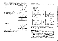
Important •Depending on the range' parameter settings, there may be some error in solutions produced by Graph Solve. *If no solution can be found for any of the above operations, the message "No solution" appears on the display. •The following conditions can interfere with calculation precision and may make it impossible to obtain a solution. *When the solution is a point of tangency to the x-axis. • *When the solution is.a point of tangency between two graphs. 8-12 Other Graph Functions The functions described in this section can be used with rectangular coordinate, polar coordinate, parametric, inequality, and statistical graphs. Important The procedures described here can be performed in the COMP, SD, REG, MAT, or TABLE Mode Or in theGRAPH Mode. The following examples show operation for the COMP Mode only. •To determine the values of points of intersection Example To determine the values of the points of intersection for the following equations: Y= -x + 2 Use the following range parameters: >jinn: - max: sc1:1 Ymin: -10 max:10 wsrcfi1rG:2 Draw the graph of the first equation. LI(SET)E(REC) IIM El(CLS)® •Setting the Type of Graphing Method (G-type) You can use the set up display to specify either of the following two graphing methods by changing the G-type setting (page 22). El(CON) 1 g(PLT) Connects plotted points with lines Only points are plotted (without connection) Overdraw the graph of the second equation. HEM ES IlTrace Function . The Trace FUnction lets you move a pointer along the line in a graph and display coordinate values at any point. The following illustrations show how values are displayed for each type of graph. IX:MS.95Y1=404.S1IBB23E •Rectangular Coordinate Graph *Polar Coordinate Graph *Parametric Graph •Inequality Graph -194- 11z-0.996931 Or-3.169311 I I Yr-0.664541 gg;1196111 'X=2.42Y5
-
 1
1 -
2
-
3
-
4
-
5
-
6
-
7
-
8
-
9
-
10
-
11
-
12
-
13
-
14
-
15
-
16
-
17
-
18
-
19
-
20
-
21
-
22
-
23
-
24
-
25
-
26
-
27
-
28
-
29
-
30
-
31
-
32
-
33
-
34
-
35
-
36
-
37
-
38
-
39
-
40
-
41
-
42
-
43
-
44
-
45
-
46
-
47
-
48
-
49
-
50
-
51
-
52
-
53
-
54
-
55
-
56
-
57
-
58
-
59
-
60
-
61
-
62
-
63
-
64
-
65
-
66
-
67
-
68
-
69
-
70
-
71
-
72
-
73
-
74
-
75
-
76
-
77
-
78
-
79
-
80
-
81
-
82
-
83
-
84
-
85
-
86
-
87
-
88
-
89
-
90
-
91
-
92
-
93
-
94
-
95
-
96
-
97
-
98
-
99
-
100
-
101
-
102
-
103
-
104
-
105
-
106
-
107
-
108
-
109
-
 110
110 -
 111
111 -
 112
112 -
 113
113 -
 114
114 -
 115
115 -
 116
116 -
 117
117 -
 118
118 -
 119
119 -
 120
120 -
121
-
122
-
123
-
124
-
125
-
126
-
127
-
128
-
129
-
130
-
131
-
132
-
133
-
134
-
135
-
136
-
137
-
138
-
139
-
140
-
141
-
142
-
143
-
144
-
145
-
146
-
147
-
148
-
149
-
150
-
151
-
152
-
153
-
154
-
155
-
156
-
157
-
158
-
159
-
160
-
161
-
162
-
163
-
164
-
165
-
166
-
167
-
168
-
169
-
170
-
171
-
172
-
173
-
174
-
175
-
176
-
177
-
178
-
179
-
180
-
181
-
182
-
183
-
184
-
185
-
186
-
187
-
188
-
189
-
190
-
191
-
192
-
193
-
194
-
195
-
196
-
197
-
198
-
199
-
200
-
201
-
202
-
203
-
204
-
205
-
206
 |
 |
