Home » Brother International Manuals » Typewriters » Brother International WP7550JPLUS » Manual Viewer

Brother International WP7550JPLUS Owner's Manual - English - Page 106

Inputting, range

Get Brother International WP7550JPLUS PDF manuals and user guides

View all Brother International WP7550JPLUS manuals

Add to My Manuals
Save this manual to your list of manuals

Page 106 highlights

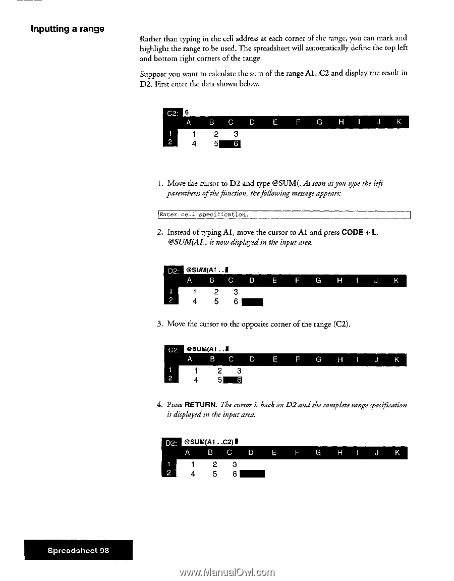
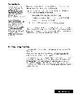
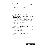
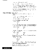
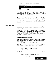
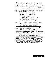
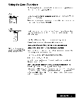
Inputting a range Rather than typing in the cell address at each corner of the range, you can mark and highlight the range to be used. The spreadsheet will automatically define the top left and bottom right corners of the range. Suppose you want to calculate the sum of the range Al ..C2 and display the result in 12$2. First enter the data shown below. C2: 6 A BC D E F G HI J K 2 3 2 4 56 1. Move the cursor to 132 and type @SUM(. As soon as you type the left parenthesis ofthefunction, thefollowing message appears: Enter cell specification. 2. Instead of typing Al, move the cursor to Al and press CODE + L. @SUM(Al.. is now displayed in the input area. D2: @SUM(A1 ..1 A C D E F G HI J K 1 2 3 2 4 56 3. Move the cursor to the opposite corner of the range (C2). C2: @SUM(A1 A BC D E F G HI J K 1 2 3 2 4 56 4. Press RETURN. The cursor is back on D2 and the complete range specification is displayed in the input area. D2: @SUM(A1 ..C2), A B 1 1 23 4 56 E F G HI J K Spreadsheet 98

Section	Page
Front Cover	1
FCC Notice	2
Table of Contents	3
1 Getting Started	9
How to Use This Manual	9
Parts of Your Whisperwriter	10
Main Unit	10
Monitor	11
Optional Modem	11
Precautions	12
Set Up	13
Attaching the Monitor Stand	13
Connecting the Equipment	14
Feeding Paper	15
Manual Paper Feeding (no cut sheet feeder)	15
Optional CF-710 Cut Sheet Feeder	16
Installing the Optional Cut Sheet Feeder	16
Automatic Papaer Feeding (with cut sheet feeder)	18
Precautions when Using the Cut Sheet Feeder	19
Manual Paper Feeding (with cut sheet feeder)	20
Removing the Optional Cut Sheet Feeder	21
Resinstaling the Paper Support	22
Ink-Jet Cartridge	22
Installing/Replacing an Ink-Jet Cartridge	23
Installing the first Ink-Jet Cartridge	23
Replacing a used Ink-Jet Cartridge	24
Cleaning the Print Head	26
Cleaning the Print Cartridge Nozzles and Contacts	26
CLeaning the Bracket Contacts in the Printer	27
Diskettes	28
Inserting and Removing a Diskette	28
Initializing (Formatting) New Diskettes	29
Write-Protecting Your Diskettes	30
Backing Up a Diskette	30
Keyboard	31
Character Keys and Cursor Keys	31
Keypad Keys	32
Function Keys	33
Operation Overview	34
Main Menu Screen	34
Application Description	34
Starting an Application	35
Function Menus	35
Dual Display	35
Clip Baord	36
Help Windows	36
Supplemental Programs	36
Self-Demo	36
Tutorial	36
Graphic Art Print (WP-7550J-Plus only)	36
Frame Print (WP-7550J-Plus only)	36
2 Word Processing	39
Starting Word Processing	39
Creating a New File	39
Editing an Existing File	39
The Input/Edit Screen	40
Basic Typing	42
Word Wrap Function	42
Hyphen Function	42
Types of Spaces	42
Paragraph Break	43
Page Break	43
Tab and Paragraph Indent	43
Typing Different Characters	43
Basic Editing	45
Cursor Movement	45
Inserting Text	46
Deleting Text	46
Using the File Functions	46
Tips for Using Files	47
Open File	47
Save File	48
Open File for Dual	48
Quit	49
Close File	50
Saving a File	50
File Name Convertions	50
File Management	51
Using the Edit Functions	52
Centering	52
Right Margin Flush	53
Justify	53
Search	54
Replace	55
Header/Footer	56
Editing Headers and Footers	56
Auto Page Numbering	56
Style	57
Hyphen Scan	57
Merge Code	58
Using the Merge Code Function	59
Insertig Merge Symbols in your Document	59
Using the Style Functions	60
Type Style Change	60
Font and Size	61
Margins and Tabs	62
Using tabs to create a table	63
Using a tab to create a Paragraph indent	63
Using a tab to create a line indent	63
Line Spacing	64
Multi-Column	64
Typing text in multi-column pages	65
Copy Format	66
Delete Format	66
Page Setup	66
Using the Block Functions	68
Move	68
Copy	69
Delete	69
Copy to/ Paste from Clip Board	70
Type Style Change / Type Style Add / Font and Size	70
Using the Graphics Functions	71
Create New Chart	71
Deleting Data	72
Chart Examples	73
Final points	75
Edit Chart	75
Line Framing	76
Editing a frame	77
Copy Graphic	78
Delete Graphic	78
Using the Option Functions	79
Abbreviated Phrase Maintenance	79
Understanding the Abbreviated Phrase Memory	79
Creating and editing an Abbreviated Phrase File	80
Check All	82
Misspelled words	82
Redundant words	84
Capitalization mistakes	84
Check During Typing ON/OFF (Spell Check)	84
User Dictionary Maintenance	84
Understanding the User Dictionary	84
Adding a word to the User Dictionary	85
Editing the User Dictionary	86
Auto Letter Layout	87
Type Thesaurus	87
Edit Thesaurus	88
Using the Screen Functions	89
Change Screen	89
Scale Line ON/OFF	89
Function Mark ON/OFF	89
Split Size	89
Using the Print Functions	91
Printing a Document	91
Using Layout to Preview a Document	93
3 Spreadsheet	95
What is a Spreadsheet	95
Starting the Spreadsheet Application	96
The Input/Edit Screen	97
Moving Around the Screen	98
Entering and Editing Data	99
Inputing Alphanumeric and Numeric Data	100
Format Marks	101
Maximum Length of Data	101
Performing Calculations	102
Direct Numbers	102
Formulas	103
Order of Calculation of a Formula	104
Using Math Functions	105
Range of cells	105
Inputing a range	106
Spreadsheet Functions	107
Using the Menu Functions	111
File	111
Edit	111
Left	112
Center	112
Right	112
Search and Replace	112
Fill	113
Sort	113
Select	114
Style Functions	117
Style notes	117
Underline	118
Bold	118
Fixed	119
Currency	119
Percent	120
Formula Text	121
No Display	121
All Off	122
Block Functions	122
Absolute and relative adddresses	122
Move	123
Copy (a range of cells)	123
Copy (one cell to other cells)	124
Clear	125
Copy to Clip Board / paste from the Clip Board	125
Sheet Functions	126
Column Width	126
Title	128
Insert	129
Delete	130
Recalc	131
Range Protect	131
Worksheet Protect	132
Calculation Method	132
Options	134
Abbreviated Phrase Maintenance	134
Check All	134
User Dictionary Maintenance	134
Screen Functions	135
Change Screen	135
Split Size	135
Print Functions	136
Setting the Print Options	136
Print Area	136
Print Point	137
Print Quality	137
Print Frozen Title	137
Cut Sheet Feeder	137
Page Setup	137
Printing	138
4 Addressbook	139
Starting Addressbook	139
Addressbook Screens	140
The View Screen	140
The Data Input Screen	141
Working with Addressbook	141
File	141
The Input Funcitons (View Screen)	142
New Record	142
Top Record	142
Bottom Record	142
The Record Functions (View Screen)	142
Move	143
Copy	143
Delete	144
Copy to Clip Board / Paste from Clip Board	144
Insert	144
The Label Functions (View Screen)	144
Insert Label	145
Delete Label	145
Chanage Label Name and Width	146
The Edit Functions (View Screen)	146
Sort Records	146
Select records	147
The Screen Function (View Screen)	148
The Print Function (View Screen)	148
Printing Labels	148
Changing label settings	150
Printing a list	150
Changing Page Setup	151
Changing label print settings	152
To start printing	152
To Stop Printing	153
Selecting records for merge printing	153
The Jump Functions (Data Input Screen)	154
Search	154
The Label Functions (Data Input Screen)	155
The Option Functions (Data Input Screen)	155
The Screen Function (Data Input Screen)	155
Return to View Screen	155
5 Template	157
Opening a Template File	157
6 Typewriter	159
Starting the Typewriter application	159
Input / Edit screen	160
Hot Zone	161
Basic Typing	161
Edit Functions	161
Auto Return On / Off	162
Find Position	162
Style Functions	163
Options Functions	163
Feeder Function	163
Exit Funciton	164
7 Communication	165
About Modems	165
Using Communications	166
Using a Communication Parameter File	167
Opening a Communication File	167
About Communications Files	168
Communication Functions	169
File Functions	169
CompuServe	169
New Set Up	171
Open File	173
Save File	174
Quit	175
Phone Functions	175
Dial	176
Auto Log-In	177
Recording Auto Log-In	177
Executing Auto Log-In	178
Disconnect	178
Transfer Functions	178
Send WP Text	178
Receive ASCII File	180
Character Code Table	183
Transmitting Control Codes	184
8 File Management	187
Starting the File Management Application	187
Making a Backup Copy of a Diskette	189
File Functions	190
File Copy	190
File Delete	191
Rename	191
Retrun to Main Menu	192
Disk Functions	193
Delete All (Diskettee Delete)	193
Initialize Disk	193
Directory Read	194
Convert Functions	195
Converting Brother Word Processing Files to a PC Format	195
Converting PC Text Files to Brother Word Processing Files	197
Converting Spreadsheet Files into Lotus 1-2-3 Files	199
Converting a Lotus 1-2-3 File into a Spreadsheet File	200
IBM PC Code	201
9 Disk Application	203
Using Graphic Art Print (WP-7550J Plus only)	203
Using Frame Print (WP-7550J Plus only)	206
Tutor / Self Demo	208
10 Auto Letter Layout	209
Creating the Letter	209
Applying Auto Letter Layout	211
From the Word Processor Application	211
From the Main Menu	212
11 Desk Top Reference ( WP-7550J Plus & WP-7550J only)	215
Starting Desk Top Reference	215
Word Reference	216
Jumble	218
User Dictionary Maintenance	219
12 Calculator	221
Starting the Calculator	221
Using Number Lock Mode (NUM LOCK)	221
Inputting Data	222
Order of Calculation	222
Maximum Length of numbers and precision	222
Storing a constant	223
Clearing	223
Returning to the Current Application	223
13 Clip Board	225
Copying Data to the Clip Board	225
Pasting Data from the Clip Board	226
Copy/Paste from Word Processing to Word Processing	227
Copy/Paste from Spreadsheet to Word Processing	227
Copy/Paste from Addressbook to Word Processing	227
Copy/Paste from Word Processing, Addressbook to Spreadsheet	228
Copy/Paste from Spreadsheet to Spreadsheet	228
Copy/Paste from Word Processing or Spreadsheet to Addressbook	228
Copy/Paste from Addressbook to Addressbook	228
Appendix	229
100 Graphic Art Images	229
100 Graphic Art Images	230
Extra character Table	234
Symbol table	234
Troubleshooting	235
Error messages	236
Specifications	237
Compatible accessories	237
Glossary	239

Match case Limit results 1 per page

Inputting

range

Rather

than

typing

the

cell

address

each

corner

the

range,

you

can

mark

and

highlight

the

range

used.

The

spreadsheet

will

automatically

define

the

top

left

and

bottom

right

corners

the

range.

Suppose

you

want

calculate

the

sum

the

range

..C2

and

display

the

result

12$2.

First

enter

the

data

shown

below.

C2:

Move

the

cursor

132

and

type

@SUM(.

soon

you

type

the

left

parenthesis

the

function,

the

following

message

appears:

Enter

cell specification.

Instead

typing

Al,

move

the

cursor

and

press

CODE

@SUM(Al..

now

displayed

the

input

area.

D2:

@SUM(A1

..1

Move

the

cursor

the

opposite

corner

the

range

(C2).

C2:

@SUM(A1

Press

RETURN.

The

cursor

back

and

the

complete

range

specification

displayed

the

input

area.

D2:

@SUM(A1

..C2),

Spreadsheet